Late last year, I proposed a model for kicking accuracy in Australian Football. This is using data from https://www.statsinsider.com.au/. In particular, I will be using data that goes into their AFL Shot Charting Explorer.
Today I will be extending the model by accounting for a few more categories of data that we have:
D<-Data[Data$`Shot type`=="Set shot",]
unique(D$`Shot result`)
[1] "Goal"                 "Behind"
[3] "Didn't make distance" "Miss, out of bounds"
[5] "Miss, in play"        "Touched"
[7] "Free kick mid-shot"
So other than “Free kick mid-shot”, which I assume is due to some kind of off-the-play violation, the remaining outcomes are
- “Goal” indicates that a goal was scored (6 points)
- “Behind” indicates that a behind was scored (1 point)
- “Miss, out of bounds” indicates that the kick went the distance, but the angle was off
- “Miss, didn’t make the distance” indicates that the kick fell short
- “Miss, in play” I am assuming is a similar outcome to “Didn’t make the distance”
- “Touched” indicated that the ball was touched before it passed through the goal posts (so it is worth 1 point rather than 6). I will code this the same as “Miss, didn’t make the distance”, as for it to be touched, the ball must have been relatively low to the ground near the goal.
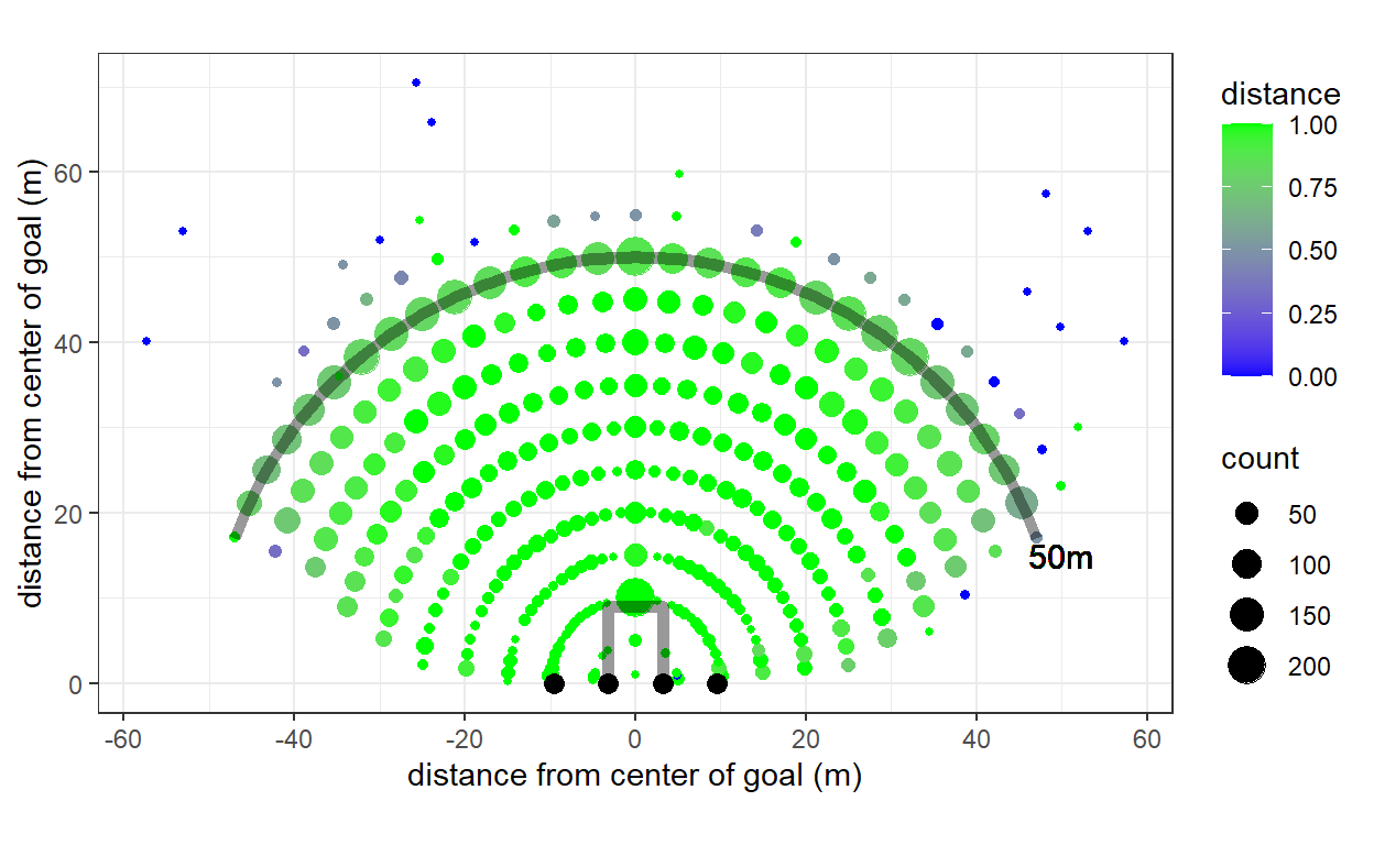
Previously, I just dropped everything except for the first three outcomes, which is probably a bit dodgy. So here are the empirical accuracies from each of the recorded locations of set shots. Here “distance” is the fraction of shots from that location that made the distance (i.e. went out of bounds or through the goal posts).
Let’s develop a model to account for these outcomes differently.
Let \(D\) be a random variable describing the actual distance of a kick (i.e. not the required distance).

To make the math easier (at the expense of a bit of realism), let’s assume that getting the distance right is not a function of a player’s error in kicking angle (the geometry of this is just wrong, maybe I will incorporate it later). This means that if a player’s kicking distance \(D\sim F_D\), then the “Miss, didn’t make the distance” events occur with probability \(F_D(r)\), where \(r\) is the distance from the kick to the center of the goal. Hence, the probability of the four possible (mutually exclusive) outcomes that I will be considering are: \[ \begin{aligned} \Pr(&\text{Miss, didn't make the distance}\mid r,\theta,\kappa,\delta,\nu)\\&=F(r;\delta)\\ \Pr(&\text{Goal}\mid r,\theta,\kappa,\delta,\nu)\\&=(1-F(r;\delta))\left[1-2\mathrm t\left(-\frac{a(qr)}{2\kappa},\nu\right)\right]\\ %% \Pr(&\text{Behind} \mid r,\theta,\kappa,\delta,\nu)\\ &=(1-F(r;\delta))\left[ \mathrm t\left(-\frac{a(qr)}{2\kappa},\nu\right)+t\left(-\frac{a(qr)}{2\kappa}-\frac{a(pq)}{\kappa},\nu\right) t\left(\frac{a(qr)}{2\kappa}+\frac{a(rs)}{\kappa},\nu\right) -t\left(\frac{a(rs)}{2\kappa},\nu\right) \right]\\ %% \Pr(&\text{Miss, out of bounds}\mid r,\theta,\kappa,\delta,\nu)\\ &=(1-\Pr(\text{Miss, didn't make the distance}\mid r,\theta,\kappa,\delta,\nu))(1-\Pr(\text{Goal}\mid r,\theta,\kappa,\delta,\nu)-\Pr(\text{Behind} \mid r,\theta,\kappa,\delta,\nu)) \end{aligned} \] where \(t(x,\nu)\) is the cdf of Student’s \(t\) distribution with \(\nu\) degrees of freedom, \(r\) and \(\theta\) measure distance to goal and angle to goal, respectively, and \(\delta\) is the parameter governing the distribution of kicking distance. \(a(pq)\) is the angle \(pxq\) (i.e. the angle between the kicker and the left two posts). I derived the expressions for the probabilities of goals and behinds, conditional on the kick making the distance, in this previous post
Let’s assume that a kick has range \(D\sim\mathrm{lognormal}(\delta_1,\delta_2)\), and so now we have the following model in Stan:
// saved as AFLAngleT.stan
data {
  vector[2] priork;
  vector[2] priornu;
  vector[3] priorDistance;
  int n;
  vector[n] goal;
  vector[n] behind;
  vector[n] MissShort;
  vector[n] bounds;
  vector[n] aGoal;
  vector[n] aLBehind;
  vector[n] aRBehind;
  vector[n] dist;
}
transformed data {
    vector[n] ones;
    for (ii in 1:n) {
        ones[ii] = 1;
    }
}
parameters {
  real<lower=0> k;
  real<lower=0> nu;
  real ldm;
  real<lower=0> ldsd;
}
transformed parameters {

}
model {
    vector[n] pGoal;
    vector[n] pLBehind;
    vector[n] pRBehind;
    vector[n] pDistance;


    // prior
    k ~ lognormal(priork[1],priork[2]);
    nu ~ lognormal(priornu[1],priornu[2]);
    ldm ~ normal(priorDistance[1],priorDistance[2]);
    ldsd ~ exponential(priorDistance[3]);


    // student_t_cdf(reals y, reals nu, reals mu, reals sigma)
    for (ii in 1:n) {
        pGoal[ii]       = student_t_cdf(aGoal[ii] / (2.0),nu,0.0,k)-student_t_cdf(-aGoal[ii] / (2.0),nu,0.0,k);
        pLBehind[ii]    = student_t_cdf(-aGoal[ii]/(2.0),nu,0.0,k)-student_t_cdf(-aGoal[ii]/(2.0)-aLBehind[ii],nu,0.0,k);
        pRBehind[ii]    = student_t_cdf(aRBehind[ii]+aGoal[ii]/(2.0),nu,0.0,k)-student_t_cdf(aGoal[ii]/(2.0),nu,0.0,k);
        pDistance[ii] = normal_cdf(log(dist[ii]),ldm,ldsd);
    }


    // likelihood contribution for goals
    target += goal .* log(pGoal .* (1.0-pDistance));
    // likelihood contribution for behinds
    target += behind .* log((pLBehind+pRBehind)  .* (1.0-pDistance));
    // likelihood contribution for miss, didn't make the distance
    target += MissShort .* log(pDistance);
    target += bounds .* log((1.0-pDistance) .* (1.0-pGoal - pRBehind-pLBehind));

    // old code for G/B/other
    // likelihood contribution for goals
    //target += goal .* log(pGoal);
    // likelihood contribution for behinds
    //target += behind .* log((pLBehind+pRBehind));
    // likelihood contribution for the rest
    //target += (MissShort+bounds) .* log(1.0-pLBehind-pRBehind-pGoal);
}

generated quantities {

}
which produces the following results:
| mean | se_mean | sd | 2.5% | 97.5% | n_eff | Rhat | |
|---|---|---|---|---|---|---|---|
| k | 0.0698231 | 0.0000245 | 0.0010919 | 0.0677675 | 0.0720713 | 1989.142 | 1.0002178 |
| nu | 7.4749125 | 0.0184609 | 0.7956717 | 6.1443187 | 9.2176177 | 1857.633 | 1.0003710 |
| ldm | 4.3545964 | 0.0006638 | 0.0285137 | 4.3014195 | 4.4136017 | 1844.933 | 1.0009109 |
| ldsd | 0.4727015 | 0.0005644 | 0.0238907 | 0.4287772 | 0.5233659 | 1791.730 | 1.0012361 |
| lp__ | -9832.0675061 | 0.0382011 | 1.4219847 | -9835.5459986 | -9830.3094180 | 1385.598 | 0.9999962 |
The parameters added since my previous post on this are “ldm” and “ldsd”, which govern the distribution of \(D\), kicking distance. Let’s have a look at what this implies about kicking range:

So now let’s have a look at what this means for the expected vale of shots from particular positions:
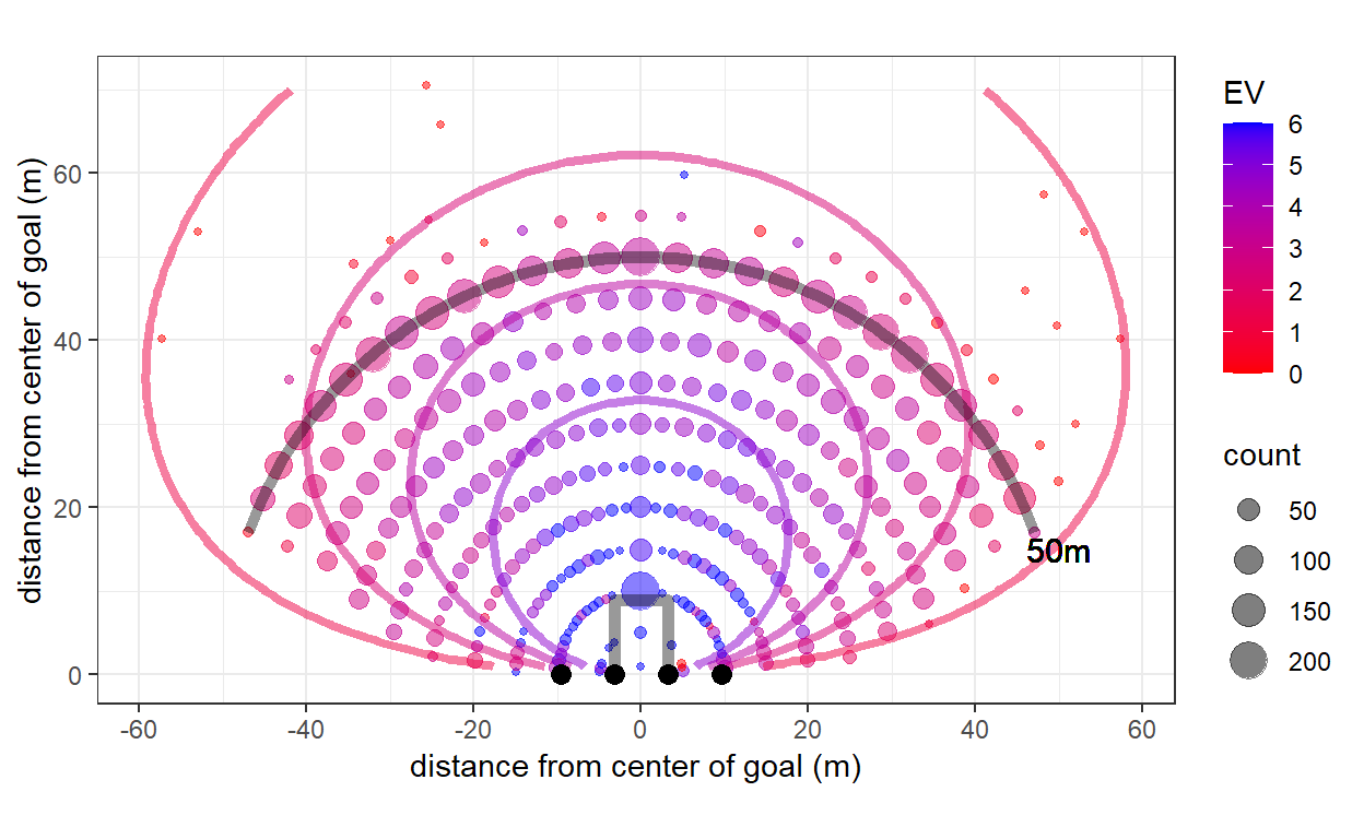
In this plot, the color shows the expected value of a set shot. The dots show empirical values (i.e. taking the average points scored from each position), and the contours show the model’s predictions. That is, shots along each contour have the same expected value. places where the contours and dots have similar colors are where the model is doing well.
I will leave this here for now, but I am certainly not done with this dataset!
BTW, I am going to be writing all of my posts here from now on, but if you want to see my older posts, they can be found on my google site