With pi day just 11 days away, it was fitting that one of my econometrics students read about approximating π using Monte Carlo simulation. Here one way to do it.
Imagine you are throwing darts at a square board with side length \(2r\). Inside this square is a circle with radius \(r\). (here I’m setteing \(r=1\)).
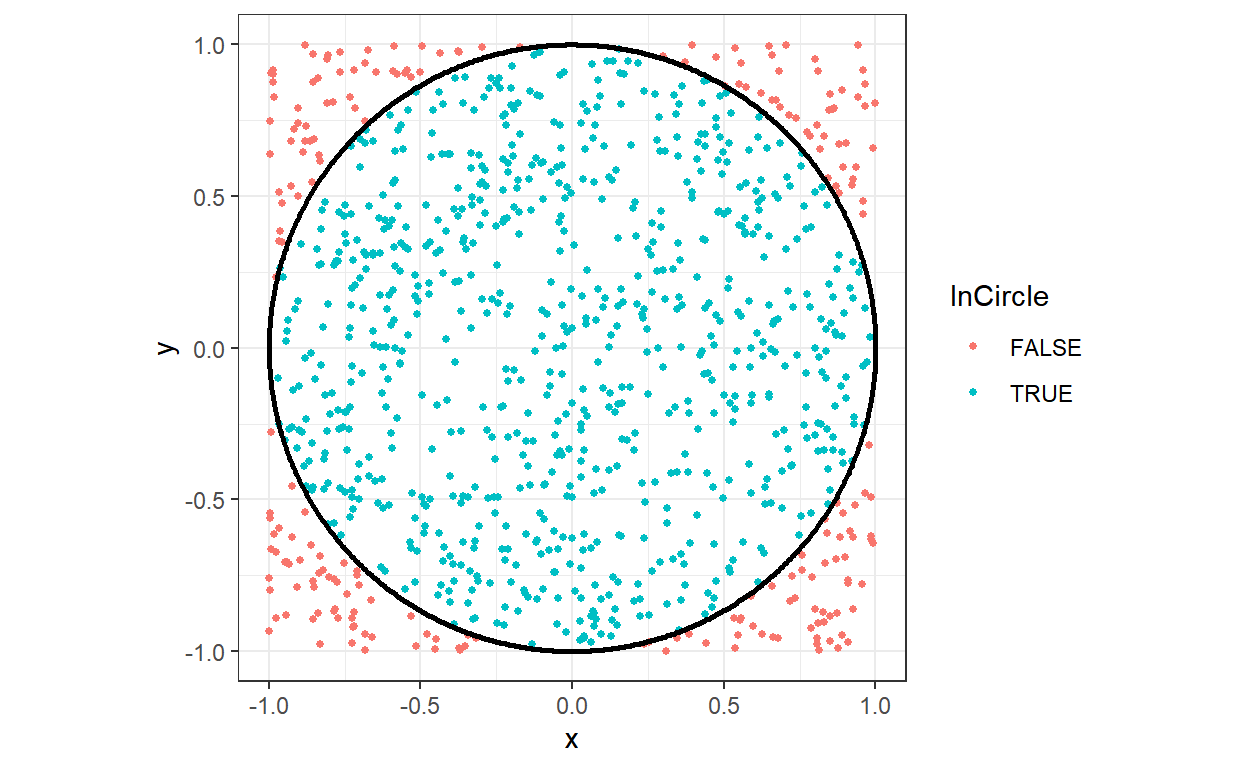
If your darts are uniformly distributed across the board, then the probability that a dart lands in the circle is: \[ \Pr\left(\text{dart in circle}\right) = \frac{\text{area of circle}}{\text{area of square}}=\frac{\pi r^2}{4r^2}=\frac{\pi}{4} \]
Hence, our approximation of pi is \(\hat\pi = \frac{4}{S}\sum_{s=1}^Sc_s\), where \(S\) is the simulation size, and \(c_s\) is an indicator variable equal to one if simulated dart \(s\) lands in the circle, and zero otherwise.
S<-1000000 # simulation size
x<-runif(S)*2-1
y<-runif(S)*2-1
d<-data.frame(x,y)
d$InCircle<-as.integer(sqrt(d$x^2+d$y^2)<1)

piApprox<-mean(d$InCircle)*4
piApprox
[1] 3.141012Compared to the actual (to my computer’s displayed precision):
pi
[1] 3.141593As with any simulation, we’re always going to be at least a little bit off, and maybe it’s even worse than that, especially if the simulation size \(S\) is small (although fixing that is a problem for my computer, not me).
How much benefit do we get by increasing the simulation size? We can answer this by recognizing that variable \(C_s\) is destributed \(\mathrm{Bernoulli}(\pi/4)\), which has mean \(\pi/4\) and variance \(\pi/4(1-\pi/4)\). And so, using the Lindeberg–Lévy Central Limit Theorem: \[ \sqrt{S}(\hat\pi-\pi)\xrightarrow[]{d} N\left(0,\pi/4(1-\pi/4)\right) \]
Note that since I am approximating \(\pi\), I probably shouldn’t use it’s value to work out the variance of \(\hat\pi\). Instead, note that \(p(1-p)\) is maximized at \(p=0.5\), so the asymptotic variance can be at most 0.25 (i.e. if \(\pi\) were exactly two). Hence, the variance of \(\hat\pi\) must satisfy (approximately, because of the \(\xrightarrow[]{d}\) part): \[ V[\hat\pi]\leq \frac{1}{4S} \]
So, for example, if we wanted to have a 95% chance (at least, due to the inequality) of being within 0.0001, we need a simulation size that satisfies:
\[ \begin{aligned} 0.0001&=1.96\sqrt{\frac{1}{4S}}\\ \left(\frac{0.0001}{1.96}\right)^2&=\frac{1}{4S}\\ S&=\frac{1.96^2}{0.0001^2\times4} \end{aligned} \]
1.96^2/(0.0001^2*4)
[1] 96040000which is almost 100 times larger than the simulation I ran above. This method isn’t particularly efficient!
I am going to be writing all of my posts here from now on, but if you want to see my older posts, they can be found on my google site