Yesterday a colleague asked me about the Ramsey RESET test. A student had asked her about whether it could be used to test for omitted variables. Specifically, whether this test could be used to determine whether an explanatory variable is endogenous.
The short answer to this question is a resounding no, but it got us thinking about the disctinction between two kinds of omitted variables:
- The kind we usually worry about, which are the ones that never show up in our dataset. These are what we usually think about when one of our explanatory variables is endogeneous.
- A transform of one of the variables we include. For example if we only include \(x\) linearly in our specification, then we are leaving out \(x^2\), \(x^3\), \(\log x\), \(x^{-1}\), \(\exp(x)\), and so on.
Unsurprisingly, the test is designed to pick up (2), and (1) is something we can never test for (outside of experiments). But I can understand why this student saw parallels between RESET and endogeneity. Let’s take a deeper dive
What is RESET?
RESET asks if the residuals from your regression have significant explanatory power for your dependent variable. Specifically, if you estimate the equation using OLS:
\[ y_i=\beta_0+\beta_1x_i+\epsilon_i \]
then if the model is correctly specified, then estimating this again by adding a polynomial of residuals from the first model on the right-hand side should not get you any better explanatory power. That is, after estimating the model above, we have residuals \(\{\hat y_i\}_{i=1}^N\), and we include powers of these on the right-hand-side:
\[
y_i=\alpha_0+\alpha_1x_i+\gamma_1\hat y^2_i+\gamma_2\hat
y_i^3+\ldots+\epsilon_i
\] then all of the \(\gamma\)
terms should be zero. This is very easy to implement in R using
the resettest function in the lmtest
package.
A simulation with misspecified functional form
When does this perform well (or as expected)? That happens when what we’re missing from our specification is a more complex relationship between \(x\) and \(y\). Here is a data-generating process that does this:
\[ \begin{aligned} y_i&=x_i+0.5x_i^2+\epsilon_i\\ x_i, \epsilon_i&\sim iid N(0,1) \end{aligned} \] That is, suppose we estimate a model including \(x\) linearly on the right-hand side. What kind of relationship do we get. Let’s simulate one sample to find out:
library(tidyverse)
set.seed(42)
N<-1000

x<-rnorm(N)
y<-x+0.5*x^2+rnorm(N)

d<-tibble(y,x)

(
  ggplot(data=d,aes(x=x,y=y))+theme_bw()
  +geom_point(alpha=0.5)
  +geom_smooth(method="lm",formula="y~x")
  +geom_abline(slope=1,intercept=0,linetype="dashed")
)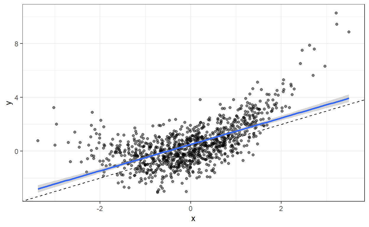
actually this model doesn’t do a bad job of picking up that \(\beta_1=1\) because the squared term is symmetric around zero, and so is the distribution of \(x\). That is why we get a line of best fit close to parallel with the \(45^\circ\) line (dashed line).
But is is clearly a bad fit. Not to worry, we can work out that we have this kind of omitted variable using RESET:
    RESET test

data:  y ~ x
RESET = 572.75, df1 = 1, df2 = 997, p-value < 2.2e-16
So we reject the null, which is good in this case because the null is false: the simple bivariate model is mis-specified because we have not included the \(x^2\) term.
A simulation with endogeneity
OK, but what about the other kind of omitted variable? To me, at least, when somebody says “omitted variable” I typically think of a variable that is not included in the model, and that practically can’t be included in the model because it is not in our data.
For this part, let’s use the classic endogeneity example of estimating the causal effect of education on wages. Here ability is the confounding, omitted, variable.
Let’s assume that the true model is:
\[ \begin{aligned} \mathrm{wage}_i&=\beta_0+\beta_1\mathrm{education}_i+\beta_2\mathrm{ability}_i+\epsilon_i\\ \mathrm{education}_i&=\gamma_0+\gamma_1\mathrm{ability}_i+\eta_i \end{aligned} \]
We will set \(\beta_0=\gamma_0=0\), \(\beta_1=\beta_2=\gamma_1=1\) for simplicity, let \(\epsilon_i,\eta_i\sim iid N(0,1)\), and education and ability are also standard normal.
Importantly, the effect of education on wage is one. So any estimator that on average gets us something other than one is biased.
Here is some code that draws from this distribution:
set.seed(42)

N<-1000 # sample size
ability<-rnorm(N)
education<-ability+rnorm(N)
wage = education+ability+rnorm(N)

d<-tibble(wage,education)

(
  ggplot(data=d,aes(x=education,y=wage))
  +geom_point(alpha=0.5)
  +geom_smooth(method="lm",formula="y~x")
  +geom_abline(slope=1,intercept = 0,linetype="dashed")
  +theme_bw()
)
Since the blue line is the line of best fit (OLS), and the dashed line has a slope of one, if we are unbiased estimating \(\beta_1\), these lines should lie on top of each other on average (or at least have the same slope).
They don’t. Why? Because the error term, call it \(u_i\), in the estimated equation includes ability:
\[ \mathrm{wage}_i=\beta_0+\beta_1\mathrm{education}_i+\underbrace{\beta_2\mathrm{ability}_i+\epsilon_i}_{u_i} \] and:
\[ \begin{aligned} \mathrm{cov}(\mathrm{education}_i,u_i) &=\mathrm{cov}(\mathrm{education}_i,\beta_2\mathrm{ability}_i+\epsilon_i)\\ &=E\left[(\mathrm{education}_i-E(\mathrm{education}_i))(\mathrm{ability}_i-E(\mathrm{ability}_i))\right]\\ &=E\left[\mathrm{education}_i\mathrm{ability}_i\right]\quad \text{(both have zero mean)}\\ &=E[(\gamma_0+\gamma_1\mathrm{ability}_i+\eta_i)\mathrm{ability}_i]\\ &=\gamma_1E[\mathrm{ability}_i^2]\\ &\neq 0 \end{aligned} \]
Here is how we can estimate the blue line:
| Dependent variable: | |
| wage | |
| education | 1.488*** |
| (0.028) | |
| Constant | -0.014 |
| (0.039) | |
| Observations | 1,000 |
| R2 | 0.741 |
| Adjusted R2 | 0.741 |
| Residual Std. Error | 1.244 (df = 998) |
| F Statistic | 2,856.708*** (df = 1; 998) |
| Note: | p<0.1; p<0.05; p<0.01 |
The RESET test includes powers of \(\hat y_i\) on the RHS of the regression. If these have significant explanatory power for \(y_i\), we reject the null of no omitted variable.
    RESET test

data:  wage ~ education
RESET = 0.0054627, df1 = 1, df2 = 997, p-value = 0.9411
so we would fail to reject the null of no omitted variables, even though the null is, by construction, false. Since the residuals are just a linear function of education, the polynomial of residuals is just a polynomial of education, which understandably has no explanatory power for wages, because I haven’t included any polynomial terms in the data-generating process.
But was I just lucky in this particular draw of data? Let’s do this 1,000 times just to be sure. To do this, I write a function that generates a sample, then outputs the slope coefficient (\(\hat\beta_1\)) of the regression, as well as the \(p\)-value of the test:
simStep<-function(N) {
  ability<-rnorm(N)
  education<-ability+rnorm(N)
  wage = education+ability+rnorm(N)
  d<-tibble(wage,education)
  reg<-lm(data=d,formula=wage~education)$coefficients["education"]
  test<-resettest(data=d,wage ~ education , power=2, type="regressor")$p.value

  c(reg,test)
}

coef<-c()
pval<-c()

for (ss in 1:1000) {
  sim<-simStep(1000)
  coef<-c(coef,sim[1])
  pval<-c(pval,sim[2])
}

simData<-tibble(coef,pval)
so we would reject the null this fraction of the time:
mean(simData$pval<0.05)[1] 0.043even though the null is false:
(
  ggplot(data=simData,aes(x=coef))
  +geom_histogram()
  +theme_bw()
  +geom_vline(xintercept=1)
)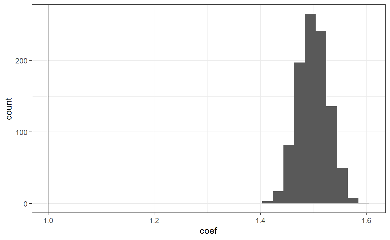
Note that rejecting the null 4.3% of the time when the null is false is a bad thing. We want to be rejecting the null here, so we recognize that we have that we have an omitted variable. In fact, we are rejecting the null about as often as we would were it true. As a Bayesian, my interpretation of this is that the test gives me absolutely no information about whether I have an omitted variable.
The trouble is that RESET isn’t trying to spot this kind of omitted variables. While it might be good for working out if you’ve got your function form right (i.e. should I include some polynomial terms?), it is not intended to alert you to an endogenous variable.