13 Application: Experience-Weighted Attraction
In this application, I will run you through my take on a Bayesian version of Table 3 of Cason, Friedman, and Hopkins (2010), which reports estimates of parameters in the Experience-Weighted Attraction model (Camerer and Ho 1999). In this experiment, participants played 80 rounds of a modification of Rock Paper Scissors called “Rock Paper Scissors Dumb”, which is shown in Table 13.1. Here the added strategy “Dumb” is never a best response to a pure strategy, but is played with probability \(\frac12\) in mixed strategy Nash equilibrium. While the games share the same mixed strategy Nash equilibrium prediction, they diverge in their predictions assuming fictitious play-like learning: in the Stable game play will converge to the Nash equilibrium, whereas in the Unstable game there will be cycles. Participants played in groups of 12, and were randomly re-matched each period with another participant in their group each round.
dStan<-readRDS("Data/CFH2010TASP/CFH2010TASP_dStan.rds")

TAB<-list(
  Unstable = dStan$payoffs[1,,],
  Stable   = dStan$payoffs[2,,]
)

for (gg in c("Stable","Unstable")) {
  colnames(TAB[[gg]])<-c("rock","paper","scissors","dumb")
  rownames(TAB[[gg]])<-c("Rock","Paper","Scissors","Dumb")
}

tab<-cbind(TAB[[1]],TAB[[2]])


tab |> kbl(caption = 'The "Unstable" and "Stable" Rock-Paper-Scissors-Dumb games. Just the payoffs of the row player are shown. The payoffs of the column player are the transpose of the row player.',booktabs=TRUE) |> kable_classic(full_width=F) |> add_header_above(c("","Unstable treatment" = 4, "Stable treatment" = 4))|
Unstable treatment
|
Stable treatment
|
|||||||
|---|---|---|---|---|---|---|---|---|
| rock | paper | scissors | dumb | rock | paper | scissors | dumb | |
| Rock | 90 | 0 | 120 | 20 | 60 | 0 | 150 | 20 |
| Paper | 120 | 90 | 0 | 20 | 150 | 60 | 0 | 20 |
| Scissors | 0 | 120 | 90 | 20 | 0 | 150 | 60 | 20 |
| Dumb | 90 | 90 | 90 | 0 | 90 | 90 | 90 | 0 |
In addition to the Stable and Unstable games, participants were also assigned either to a high payoffs or low payoffs treatment, where the “Experimental Francs” in the above table were multiplied by 0.05 and 0.02 US dollars respectively.
In their Table 3, Cason, Friedman, and Hopkins (2010) estimate several permutations of the Experience-Weighted Attraction (EWA) model (Camerer and Ho 1999). This model nests some important special cases of learning models, including Stochastic Fictitious Play (SFP), which assumes that a player’s beliefs in period \(t\) are equal to the (potentially weighted) average of empirical choice frequencies observed up to that point. As noted by Wilcox (2006) however, the EWA model suffers from heterogeneity bias: if participants are heterogeneous in their parameters, then pooled estimates of these parameters will be biased. In particular, the pooled estimator favors reinforcement learning over belief learning. Fortunately, one remedy to this is relatively straightforward and lends itself to Bayesian estimation: model the heterogeneity! As such, estimating a hierarchical model makes a lot of sense here.
13.1 The model at the individual level
The EWA model (Camerer and Ho 1999) is a 4-parameter model that describes how players form expectations about payoffs based on the history of play. These expectations about payoffs are called “attractions”, which evolve according to the following equations:
\[ \begin{aligned} A^j_{i,t}&=\frac{\phi N_{i,t-1}A_{i,t-1}^j+\left[\delta+(1-\delta)I_{j,t-1}\right]\pi_{j,t-1}}{N_{i,t}}\\ N_{i,t}&=\rho N_{i,t-1}+1 \end{aligned} \]
where:
- \(\pi_{j,t-1}\) is the payoff the payer would have received had they taken action \(j\) in the previous period. That is, it is a function of the action that their opponent took in the previous period.
- \(I_{j,t-1}=1\) iff action \(j\) was played in the previous period, zero otherwise.
This part of the model has three parameters, all of which are constrained to the unit interval:
- \(\phi\) and \(\rho\) are “recency” parameters. When both are equal to one, the participant takes a simple average of the payoffs from all previous periods (this is the fictitious play model). If they are both equal and less than one, the participant takes a weighted average of payoffs from all of the previous rounds (this is the weighted fictitious play model).
- \(\delta\) is an “imagination factor”. When \(\delta=1\) the player can “imagine” what would have happened if they played action \(j\), even if they had in fact not played action \(j\). On the other hand, when \(\delta=0\), they only consider the payoff that they get from the action they took in the previous period.
Players then probabilistically best respond to these attractions. Specifically, the probability of player \(i\) taking action \(j\) in period \(t\) follows a logit choice rule:
\[ p_{i,t}^j=\frac{\exp(\lambda A_{i,t}^{j})}{\sum_{k=1}^n\exp(\lambda A_{i,t}^{k})} \]
where \(\lambda>0\) is the choice precision parameter.
Cason, Friedman, and Hopkins (2010) set their initial conditions to \(A_{i,0}^j=1\) and \(N_{i,0}=0\), noting that their results are “robust to alternative initial attraction and experience weights” (see their footnote 8). I will stick with this assumption for my analysis.
13.2 Some computational and coding issues
While we are mostly very lucky in experiments to collect our data in a very clean format that usually requires very little tidying, sometimes we get something special. In this case, there was a tornado during one of the sessions, and so these participants only got to play the game for 70 periods, instead of the planned 80.55 This is why you will see me pass a binary variable to Stan called UseData, which tells it whether or not to let an observation contribute to the likelihood. As you will see in other examples where I use cross-validation, having a variable like UseData is generally helpful anyway, as it allows us to easily turn on or off whether or not we are using some data, without modifying our Stan program. It is also useful if we want to get draws from the prior: just set all of its elements to zero!
Perhaps more importantly for your own applications, I want you to note that there is a lot we can do here to speed up computational time by pre-processing some of the variables in the model. Specifically, the variables \(I_{j,t}\) and \(\pi_{j,t}\) do not depend on the model’s parameters, and so we can pre-calculate these before passing them to Stan, which means we only have to evaluate these once.56 This will greatly reduce the computational time compared to doing these in the model or transformed parameters block, which are evaluated thousands of times.
Also, the recursive equation specifying \(A_{i,t}^j\) means that we will not be able to avoid looping over the \(t\) dimension of this problem: we cannot compute \(A_{i,t}^j\) without knowing \(A_{i,t-1}^j\). Since there were 80 periods per participant, this could be a considerable time suck for Stan. That being said, with some careful thought to vectorization, we will be able to avoid looping over the \(i\) and \(j\) dimensions. This will greatly speed things up compared to a triple for loop. I have left my inefficient code looping over \(i\) in the Stan file for the representative agent model, commented out, to show you what the double for loop would look like. Spotting these vectorized representations of the operations we need to do will usually come in handy, and while it might not save too much time for the representative agent model, the time savings will be carried through when we are estimating the hierarchical model. As you will see in my code for the representative agent model, I don’t give a hoot about eliminating triple for loops in the transformed data block. This block will only run once, so the time savings will be negligible. On the other hand, the transformed parameters, model, and to a lesser extent generated quantities57 blocks will have to run thousands of times to get your posterior simulation, so for these blocks it is usually worth vectorizing things.
Finally, while datasets from economic experiments are not usually that big, our posterior simulations from hierarchical models can get large. This is because the augmented data will have several individual-level parameters per participant.58
While I don’t run into any RAM constraints on my laptop in running this, I do like to back all of my work up in the cloud somewhere, so you might want to think about how much you save and where it goes. There is nothing in this chapter that cannot be re-run in a day if you have to, so saving just the code to get you the estimates in the cloud may be an appropriate choice if your Dropbox is getting full. This is why I use the pars = ..., include = FALSE options when calling sampling for the hierarchical model.
13.3 Representative agent models
Let’s start with estimating some representative agent models. I do this not because we should take them as seriously as the hierarchical model, but because they are a useful stepping stone for getting us to the hierarchical model. We can also compare these to the hierarchical model to see how much heterogeneity bias we might get. Additionally, as Cason, Friedman, and Hopkins (2010) also estimate these representative agent models, I will have an opportunity to verify that my code is working correctly before going to the more complicated model.
13.3.1 Prior calibration
To begin with, let’s think about priors. We have four parameters: \(\phi\in(0,1)\), \(\rho\in(0,1)\), \(\delta\in(0,1)\), and \(\lambda\in(0,\infty)\). Since the first three are all constrained to the unit interval, a good starting place is to use the uniform distribution. In my code, I allow this to be a Beta distribution, which generalizes the uniform, but I will stick to the uniform to keep things simple.
For \(\lambda\), we want to constrain it to positive real numbers, so a log-normal distribution is appropriate: \[ \log\lambda\sim N(m_\lambda,s_\lambda^2) \] The difficulty in choosing \(\lambda\) is choosing an appropriate scale, which since we are dealing with a log-normal distribution, is as much about its median as it is about its standard deviation. Small \(\lambda\) implies choices are not very precise, so participants will not be very sensitive to the attractions \(A_{i,t}^j\). On the other hand if \(\lambda\) is large, choices will be precise, and small changes in \(A_{i,t}^j\) will imply large changes in choice probabilities. But what exactly are “small” and “large” values of \(\lambda\)? I find it helps here to plot some predicted choice probabilities over a relevant scale of payoffs. Note that in Table 13.1, the smallest payoff is zero points, and the largest payoff is 150 points. Therefore payoff differences must be in this range. Converting this to dollars by using the average of the two exchange rates, we therefore have a range of \([0,150\times 0.035]=[0,5.25]\). We can use the logit Quantal Response Equilibrium (QRE) predictions to further narrow down this scale. Fortunately in this game, computing the Quantal Response Equilibrium is really easy, because Cason, Friedman, and Hopkins (2010) derive the results for us, and it turns out that we can characterize the Quantal Response Equilibrium as \(\hat p=\begin{pmatrix}m,m,m,k\end{pmatrix}\), where \(k\in[0.25,0.5]\) and \(m = (1-k)/3\). Because there is a unique \(\lambda\) for each QRE, we can back it out once we know the equilibrium probabilities:
pD<-seq(0.25,0.5-1e-6,length=100)
ExRate<-0.035
Uunstable<-dStan$payoffs[1,,]
Ustable<-dStan$payoffs[2,,]

QRE<-tibble()
for (pp in pD) {
  p<-c(rep((1-pp)/3,3),pp)
  U<-Uunstable%*%p*ExRate
  lambda<-(log(p[1])-log(p[4]))/(U[1]-U[4])
  QRE<-rbind(QRE,
             tibble(game="Unstable",pD = pp,lambda = lambda)
             )
  U<-Ustable%*%p*ExRate
  lambda<-(log(p[1])-log(p[4]))/(U[1]-U[4])
  QRE<-rbind(QRE,
             tibble(game="Stable",pD = pp,lambda = lambda)
             )
}

(
  ggplot(QRE,aes(x=lambda,y=pD,linetype = game))
  +geom_path()
  +scale_x_continuous(trans="log10")
  +theme_bw()
  +ylab("Probability of playing 'Dumb'")
  +xlab(expression(lambda))
)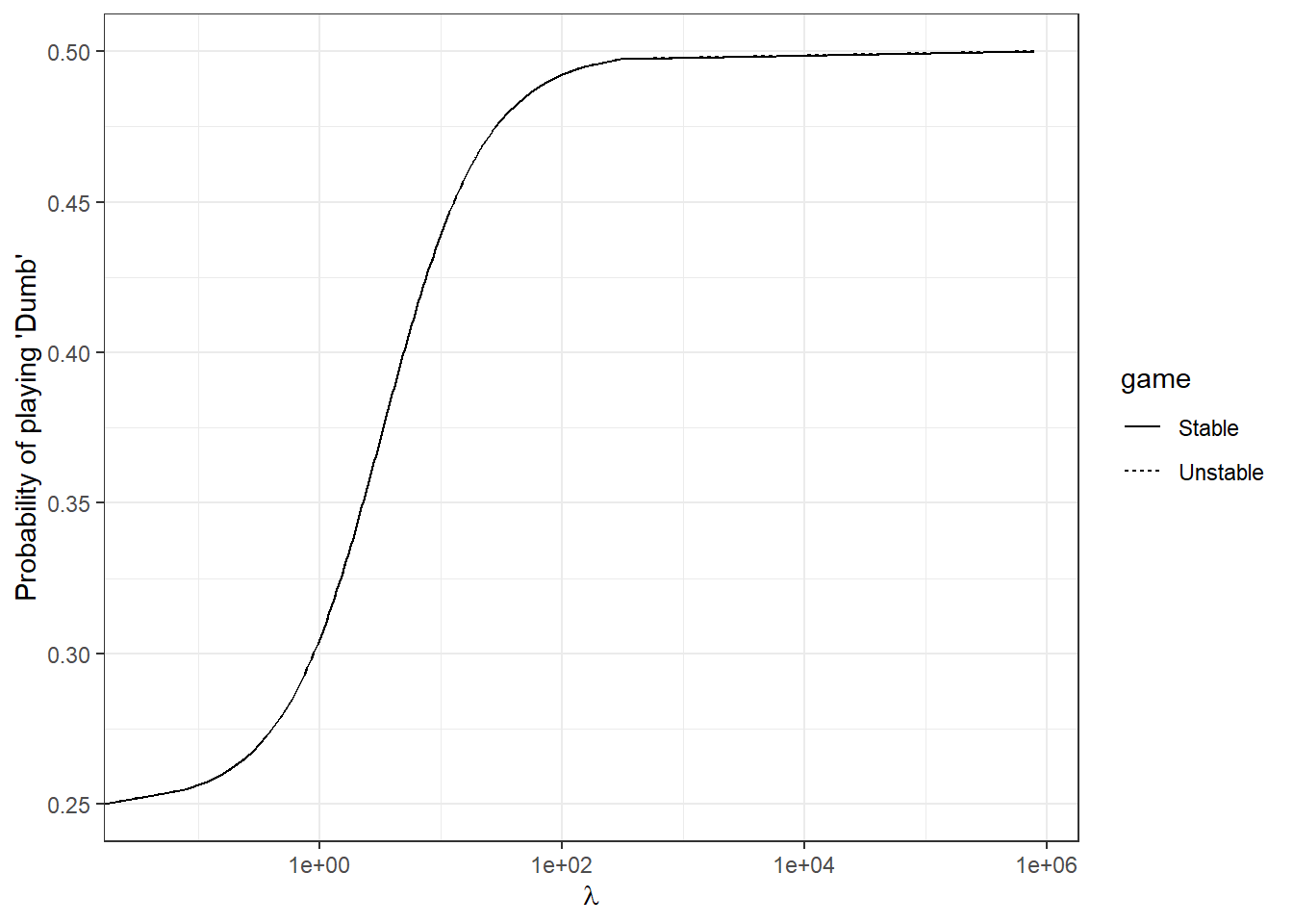
Figure 13.1: Quantal Response Equilibrium probabilities of choosing ‘Dumb’
Some things to note here:
- The Quantal Response Equilibrium probability of playing Dumb is the same for both games (this is derived in Cason, Friedman, and Hopkins (2010)). We can see this in the plot because both curves lie on top of each other.
- All of the interesting stuff seems to be happening between \(\lambda=0.1\) and \(\lambda = 100\).
Let’s target our prior so that we place 95% prior probability mass in this “interesting” range. This sets up the following system of equations:
\[ \begin{aligned} -1.96s_\lambda&=\log(0.1)-m_\lambda\\ 1.96s_\lambda&=\log(100)-m_\lambda\\ \\ m_\lambda&=\frac{1}{2}\left(\log(100)+\log(0.1)\right)\approx1.15\\ s_\lambda&=\frac{\log(100)-\log(0.1)}{2\times 1.96}\approx1.76 \end{aligned} \]
And so our prior for \(\lambda\) is:
\[ \log\lambda \sim N(1.15,1.76^2) \]
13.3.2 The Stan model
Here is the code I came up with to implement the model in Stan.
data {
  int nPeriods;
  int nParticipants;
  int nGames;
  int nActions;

  // action chosen. 1=Rock, 2=Paper, 3=Scissors, 4=Dumb
  int direction[nPeriods,nParticipants];

  // =1 if low payoffs used, =2 if high payoffs used
  int HiPay[nPeriods,nParticipants];

  // first element: low payoffs exchange rate
  // second element: high payoffs exchange rate
  real payoff_multipliers[2];

  // =1 if the observation should contribute to the likelihood
  int UseData[nPeriods,nParticipants];


  // Pre-calculated components of the EWA model
  real PI[nPeriods,nParticipants,nActions];
  real I[nPeriods,nParticipants,nActions];

  // priors
  real prior_phi[2]; // Beta
  real prior_delta[2]; // Beta
  real prior_rho[2]; // Beta
  real prior_lambda[2]; // log-normal

  real max_payoff;
}

transformed data {
  matrix[nParticipants,nActions] DIRECTION[nPeriods];

  for (tt in 1:nPeriods) {
    DIRECTION[tt] = rep_matrix(0.0,nParticipants,nActions);
    for (ii in 1:nParticipants) {
      for (aa in 1:nActions) {
        if (direction[tt,ii]==aa) {
          DIRECTION[tt][ii,aa] = 1.0;
        }
      }
    }
  }
}

parameters {

  real<lower=0,upper=1> phi; // recency
  real<lower=0,upper=1> rho; // recency
  real<lower=0,upper=1> delta; // imagination
  real<lower=0> lambda; // precision

}

model {

  // initial conditions. See CFH201 footnote 8
  matrix[nParticipants,nActions] A = rep_matrix(1.0,nParticipants,nActions);
  vector[nParticipants] N = rep_vector(0.0,nParticipants);


  for (tt in 1:nPeriods) {

    // increment the likelihood
    matrix[nParticipants,nActions] lA = lambda*(to_vector(payoff_multipliers[HiPay[tt,]])*rep_row_vector(1.0,nActions)).*(A-max_payoff);
    vector[nParticipants] lsum_lA = log(exp(lA)*rep_vector(1.0,nActions));

    /*
    Note here the for loop that would do the same thing as the uncommented line below it
    I construct DIRECTION in the transformed data block
    */

    //for (ii in 1:nParticipants) {
    //  target+= UseData[tt,ii]*(lA[tt,direction[tt,ii]]-lsum_lA[ii]);
    //}

    target+=to_vector(UseData[tt,]) .* (((lA-lsum_lA*rep_row_vector(1.0,nActions)) .* DIRECTION[tt])*rep_vector(1.0,nActions));


    // Update A and N

    matrix[nParticipants,nActions] I_t = to_matrix(I[tt,,]);
    matrix[nParticipants,nActions] pi_t = to_matrix(PI[tt,,]);

    A = (phi*(N*rep_row_vector(1.0,nActions)).*A+(delta+(1.0-delta)*I_t).*pi_t)
          ./ (rho * N * rep_row_vector(1.0,nActions)+1.0);

    N = rho*N+1.0;

  }

  // priors

  phi ~ beta(prior_phi[1],prior_phi[2]);
  rho ~ beta(prior_rho[1],prior_rho[2]);
  delta ~ beta(prior_delta[1],prior_delta[2]);
  lambda ~ lognormal(prior_lambda[1],prior_lambda[2]);

}
One thing to note from this code is that I have subtracted the variable max_payoff from all of the attractions before exponentiating them to compute choice probabilities. Mathematically this does absolutely nothing, because:
\[\frac{\exp(x-a)}{\exp(x-a)+\exp(y-a)}=\frac{\exp(x)}{\exp(y)+\exp(y)}\]
does not depend on \(a\). However this doesn’t do nothing for computing the choice probabilities. In particular, if \(x\) is large, then \(\exp(x)\) is really large, and our poor computer may have some trouble handling it. The solution I use is to subtract a large constant (i.e. the maximum payoff in the game) from all attractions. This way we are always exponentiating numbers that are less than zero. Since this is the functional form we are using for choice probabilities, we are taking logs of them when we increment the likelihood. If (in this simplified example) \(y\) is very large and positive, then exp(y) might be “rounded” to Inf, in which case the fraction becomes indistinguishable from zero, and the log-likelihood is -Inf. Keeping the numbers that we are exponentiating in a softmax small will avoid this problem. In fact, I suspect that Stan’s inbuilt softmax function will do this for you, but unfortunately in this application it did not lend itself to my vectorization of the problem.
13.3.3 Results
Here I replicate the first panel Table 3 of Cason, Friedman, and Hopkins (2010), which estimates a pooled model for each of the four treatments. I also include a fifth column pooling all of the data.
rounding<-3
RAEstimatesList<-dir(path="Code/CFH2010TASP",pattern="Estimates_RA_")
TABLE<-c()
names<-c()
for (ee in RAEstimatesList) {
  estimates<-readRDS(paste0("Code/CFH2010TASP/",ee)) |> round(rounding)
  msd<-paste0(estimates[,"mean"]," (",estimates[,"sd"],")")
  TABLE<-cbind(TABLE,msd)
  names<-c(names,ee |> str_remove("Estimates_RA_") |> str_remove(".rds"))
}
colnames(TABLE)<-names
rownames(TABLE)<-c("$\\psi$","$\\rho$","$\\delta$","$\\lambda$","lp__")
TABLE |> kbl(caption="Posterior moments (means with standard deviations in parentheses) of the representative agent models. ") |> kable_classic(full_width=F)| Pooled | StableHi | StableLow | UnstableHi | UnstableLow | |
|---|---|---|---|---|---|
| \(\psi\) | 0.909 (0.004) | 0.934 (0.006) | 0.91 (0.007) | 0.882 (0.011) | 0.888 (0.009) |
| \(\rho\) | 0.564 (0.063) | 0.437 (0.184) | 0.59 (0.106) | 0.404 (0.157) | 0.474 (0.166) |
| \(\delta\) | 0.007 (0.006) | 0.018 (0.016) | 0.012 (0.011) | 0.032 (0.023) | 0.021 (0.018) |
| \(\lambda\) | 0.355 (0.046) | 0.257 (0.082) | 0.42 (0.088) | 0.295 (0.074) | 0.365 (0.102) |
| lp__ | -12448.586 (1.498) | -3070.514 (1.575) | -3118.543 (1.622) | -3152.688 (1.551) | -3115.559 (1.617) |
Comparing this to the left panel in Table 3 of Cason, Friedman, and Hopkins (2010), these estimates are very similar. This is especially the case for \(\phi\), whose posterior means match their MLE counterparts to at least two decimal places. Since \(\rho\) is estimated with less precision than \(\phi\) in both tables, it should be unsurprising that there is less agreement between these estimates, however everything is accurate to one standard deviation/error. The biggest discrepancy is for choice precision \(\lambda\), which I estimate to be much larger than do Cason, Friedman, and Hopkins (2010). I suspect that this is due to my model using US dollars as the unit for utility, whereas it looks like Cason, Friedman, and Hopkins (2010) used experimental francs. Multiplying my estimates of \(\lambda\) by the exchange rate at least achieves estimates in the same order of magnitude as their Table 3.
13.4 Hierarchical model
So now that we have a representative agent model that works, we can move on to extending it to a hierarchical model. To modify the Stan program, we will need to:
- Convert the scalar individual-level parameters \(\phi\), \(\rho\), \(\delta\), and \(\lambda\) into vectors of length
nParticipants. - Specify the population level parameters and choose some appropriate priors for them
- Link the distribution of these individual-level parameters to the new population-level parameters.
To speed up computation, I will also use Cholesky factorization of the covariance matrix, which I discuss in the hierarchical models chapter of this book.
The hierarchical specification I will use for this model is:
\[ \begin{aligned} \begin{pmatrix} \Phi^{-1}(\phi_i)\\ \Phi^{-1}(\rho_i) \\ \Phi^{-1}(\delta_i) \\ \log (\lambda_i) \end{pmatrix}=\theta_i\sim N(\mu,\mathrm{diag\_matrix(\tau)}\Omega\mathrm{diag\_matrix(\tau)}) \end{aligned} \]
where \(\mu\) is a vector of transformed population means, \(\tau\) is a vector of standard deviations, and \(\Omega\) is a correlation matrix. The inverse normal cdf transform \(\Phi^{-1}(\cdot)\) ensures that parameters \(\phi_i\), \(\rho_i\), and \(\delta_i\) are between zero and one, and the log transform ensures that \(\lambda_i\) is positive.
Apart from the differences due to my Bayesian implementation and the MLE implementation in Cason, Friedman, and Hopkins (2010), there are few important differences in this specification:
- I permit correlation between the individual-level parameters through the correlation matrix \(\Omega\). In Table 3 of Cason, Friedman, and Hopkins (2010) these parameters are assumed to be uncorrelated
- I assume that all the individual-level parameters are heterogeneous. Note that in the middle panel of Table 3 of Cason, Friedman, and Hopkins (2010), there is not a measure of spread for parameter \(\delta_i\), whereas there is one for the other three parameters. I take this to mean that \(\delta_i\) is assumed to be constant across participants in their models.
13.4.1 Prior calibration
Here I use the normal-half Cauchy-LKJ type of prior for the population-level parameters \(\mu\) \(\tau\) and \(\Omega\) discussed in the Hierarchical Models chapter of this book. For \(\mu\), I center the priors on each parameter’s prior median from the representative agent models. For the probit-normal parameters \(\phi_i\), \(\rho_i\), and \(\delta_i\), note that the corresponding element for \(\mu\) pins down their prior medians. Setting a standard normal prior for, say, \(\mu_\phi\sim N(0,1)\) would therefore mean that our prior belief was that the median of \(\phi_i\) was uniformly distributed. As the median being very close to 0 or 1 for these parameters seems unlikely, I choose a slightly smaller prior standard deviation for these:
\[ \mu_\phi,\ \mu_\rho,\ \mu_\delta\ \sim N(0,0.25^2) \]
Similarly for \(\lambda_i\):
\[ \mu_\lambda\sim N(1.15,0.75^2) \]
centers the median of this prior over the prior we used for the representative agents model, but reduces some of its variance: our prior uncertainty about a parameter’s median should be lower than our prior uncertainty about the parameter itself.
For \(\tau\), I select:
\[ \tau_\phi,\ \tau_\rho,\ \tau_\delta,\ \tau_\lambda \sim \mathrm{Cauchy}^+(0,0.05) \]
This makes the 95th percentile of the prior distribution for each of these about 0.6. For perspective, for the log-normal distribution of \(\lambda_i\), \(\tau_\lambda=0.6\) implies that \(\lambda_i\) will be within about 31% and 320% of its population median with probability 95%. For the other, probit-normally distributed parameters, this ensures that their distributions are single-peaked.
Finally, for the prior for \(\Omega\) I choose:
\[ \Omega \sim \mathrm{LKJ}(5) \]
13.4.2 The Stan model
Here is how I modified my representative agent model to a hierarchical model. Hopefully you can see that a lot of it is exactly the same as the representative agent model. The hardest part for me came from converting all of the individual-level parameters from reals to vectors, as this meant I had to change some of the lines that calculated the attractions so that matrix sizes agreed again, and so on.59
data {
  int nPeriods;
  int nParticipants;
  int nGames;
  int nActions;

  // action chosen. 1=Rock, 2=Paper, 3=Scissors, 4=Dumb
  int direction[nPeriods,nParticipants];

  // =1 if low payoffs used, =2 if high payoffs used
  int HiPay[nPeriods,nParticipants];

  // first element: low payoffs exchange rate
  // second element: high payoffs exchange rate
  real payoff_multipliers[2];

  // =1 if the observation should contribute to the likelihood
  int UseData[nPeriods,nParticipants];


  // Pre-calculated components of the EWA model
  real PI[nPeriods,nParticipants,nActions];
  real I[nPeriods,nParticipants,nActions];

  // priors
  real prior_phi[2]; // Beta
  real prior_delta[2]; // Beta
  real prior_rho[2]; // Beta
  real prior_lambda[2]; // log-normal

  real max_payoff;

  vector[2] prior_MU[4];
  vector[4] prior_TAU;
  real prior_OMEGA;

  int nSimPars;
}

transformed data {
  matrix[nParticipants,nActions] DIRECTION[nPeriods];
  matrix[4,nSimPars] zsim;

  for (pp in 1:4) {
    for (ss in 1:nSimPars) {
      zsim[pp,ss] = std_normal_rng();
    }
  }


  for (tt in 1:nPeriods) {
    DIRECTION[tt] = rep_matrix(0.0,nParticipants,nActions);
    for (ii in 1:nParticipants) {
      for (aa in 1:nActions) {
        if (direction[tt,ii]==aa) {
          DIRECTION[tt][ii,aa] = 1.0;
        }
      }
    }
  }
}

parameters {

  vector[4] MU;
  vector<lower=0>[4] TAU;

  cholesky_factor_corr[4] L_OMEGA;

  matrix[4,nParticipants] z;


}

transformed parameters {
  vector[nParticipants] phi;
  vector[nParticipants] rho;
  vector[nParticipants] delta;
  vector[nParticipants] lambda;

  {
    matrix[4,nParticipants] theta = MU*rep_row_vector(1.0,nParticipants)+ diag_pre_multiply(TAU, L_OMEGA) * z;

    phi = Phi_approx(to_vector(theta[1,]));
    rho = Phi_approx(to_vector(theta[2,]));
    delta = Phi_approx(to_vector(theta[3,]));
    lambda = Phi_approx(to_vector(theta[4,]));

  }
}

model {

  // hierarchical structure
  to_vector(z) ~ std_normal();
  L_OMEGA ~ lkj_corr_cholesky(prior_OMEGA);
  TAU ~ cauchy(0.0,prior_TAU);

  for (pp in 1:4) {
    MU[pp] ~ normal(prior_MU[pp][1],prior_MU[pp][2]);
  }


  // initial conditions. See CFH201 footnote 8
  matrix[nParticipants,nActions] A = rep_matrix(1.0,nParticipants,nActions);
  vector[nParticipants] N = rep_vector(0.0,nParticipants);


  for (tt in 1:nPeriods) {

    // increment the likelihood
    matrix[nParticipants,nActions] lA = lambda*rep_row_vector(1.0,nActions) .*(to_vector(payoff_multipliers[HiPay[tt,]])*rep_row_vector(1.0,nActions)).*(A-max_payoff);
    vector[nParticipants] lsum_lA = log(exp(lA)*rep_vector(1.0,nActions));

    target+=to_vector(UseData[tt,]) .* (((lA-lsum_lA*rep_row_vector(1.0,nActions)) .* DIRECTION[tt])*rep_vector(1.0,nActions));


    // Update A and N

    matrix[nParticipants,nActions] I_t = to_matrix(I[tt,,]);
    matrix[nParticipants,nActions] pi_t = to_matrix(PI[tt,,]);

    A = ((phi*rep_row_vector(1.0,nActions)) .*(N*rep_row_vector(1.0,nActions)).*A+(delta*rep_row_vector(1.0,nActions)+(1.0-(delta*rep_row_vector(1.0,nActions))) .*I_t).*pi_t)
          ./ ((rho*rep_row_vector(1.0,nActions)) .* (N * rep_row_vector(1.0,nActions))+1.0);

    N = rho .* N+1.0;

  }

  // priors

  phi ~ beta(prior_phi[1],prior_phi[2]);
  rho ~ beta(prior_rho[1],prior_rho[2]);
  delta ~ beta(prior_delta[1],prior_delta[2]);
  lambda ~ lognormal(prior_lambda[1],prior_lambda[2]);

}

generated quantities {

  real mean_phi;
  real mean_rho;
  real mean_delta;
  real mean_lambda = exp(MU[4]+0.5*TAU[4]^2);

  real median_phi = Phi_approx(MU[1]);
  real median_rho = Phi_approx(MU[2]);
  real median_delta = Phi_approx(MU[3]);
  real median_lambda = exp(MU[4]);

  real sd_phi;
  real sd_rho;
  real sd_delta;
  real sd_lambda = sqrt((exp(TAU[4]^2)-1.0)*exp(2*MU[4]+TAU[4]^2));

  real CV_phi;
  real CV_rho;
  real CV_delta;
  real CV_lambda;


  matrix[4,4] OMEGA;
  OMEGA = L_OMEGA*L_OMEGA';


  {
    matrix[4,nSimPars] theta = MU*rep_row_vector(1.0,nSimPars)+ diag_pre_multiply(TAU, L_OMEGA) * zsim;

    vector[nSimPars] phi_sim = Phi_approx(to_vector(theta[1,]));
    vector[nSimPars] rho_sim = Phi_approx(to_vector(theta[2,]));
    vector[nSimPars] delta_sim = Phi_approx(to_vector(theta[3,]));
    vector[nSimPars] lambda_sim = Phi_approx(to_vector(theta[4,]));

    mean_phi = mean(phi_sim);
    mean_rho = mean(rho_sim);
    mean_delta = mean(delta_sim);

    sd_phi = sd(phi_sim);
    sd_rho = sd(rho_sim);
    sd_delta = sd(delta_sim);
  }

  CV_phi = sd_phi/mean_phi;
  CV_rho = sd_rho/mean_rho;
  CV_delta = sd_delta/mean_delta;
  CV_lambda = sd_lambda/mean_lambda;
}
If you look at the R code below implementing this estimator, I got the bulk ESS low error when running this with Stan’s default iter = 2000, where ESS stands for “Effective Sample Size”. This means that the 4,000 posterior draws60 were dependent enough that they did not provide sufficient information to accurately approximate posterior moments.
The simple fix to this, which worked for me, was just to run the chains for longer. Doubling the number of iterations to iter = 4000 fixed this.61
As mentioned above if left unchecked, this Stan fit object will take up quite a bit of space if we save all of the variables. As I don’t want to report anything on the standardized individual-level parameters \(z\), I use the pars = c("z"), include=FALSE, options in sampling, which drops these variables. What is left are the the individual-level parameters \(\begin{pmatrix}\phi_i& \rho_i & \delta_i & \lambda_i\end{pmatrix}\), and the population-level draws for \(\mu\), \(\tau\), and \(\Omega\). Even so, this produces a Stan fit object that takes up about 140MB, most of which is storing the individual-level parameters.62
13.4.3 Results
For the hierarchical model, I just estimate one model using all of the data from all four treatments. This is because I was having trouble getting Stan to estimate the treatment-specific hierarchical models without returning a divergent transitions error. I will work on fixing these errors in a future iteration of this chapter.
A summary of this model in shown in Table 13.3. One of the things I really like about the way Cason, Friedman, and Hopkins (2010) display the estimates from their hierarchical models in Table 3 is that instead of reporting the models’ fundamental population-level parameters (i.e. \(\mu\), \(\tau\), and \(\Omega\) for me), they instead focus on moments of the implied individual-level parameters. That is, they report the mean, median, and coefficient of variation (standard deviation divided by mean) for \(\phi_i\), \(\rho_i\), and \(\lambda_i\). This makes their marginal distributions much easier to interpret.
I follow suit in doing this, as well as reporting the standard deviations. As you can see in the generated quantities block of my Stan program above, these are fairly easy to compute using explicit formulas for the median and for all moments of \(\lambda_i\), which is log-normally distributed. The other parameters are probit-normally distributed, and so explicit expressions of the mean and standard deviations do not exist. I use Monte Carlo integration to evaluate these.
rounding<-3
pars<-c("phi","rho","delta","lambda")
parUnicode<-c("$\\psi$","$\\rho$","$\\delta$","$\\lambda$")
summaries<-c("mean","median","sd","CV")

param_list<-c()
param_labels<-c()
param_summaries<-c()
for (pp in 1:length(pars)) {
  for (ss in summaries) {
    param_list<-c(param_list,paste0(ss,"_",pars[pp]))
    param_labels<-c(param_labels,paste0(parUnicode[pp]))
    param_summaries<-c(param_summaries,ss)
  }
}
FitALL<-readRDS("Code/CFH2010TASP/Estimates_Hierarchical_Pooled.rds")

print(FitALL |> check_hmc_diagnostics())
##
## Divergences:## 0 of 8000 iterations ended with a divergence.##
## Tree depth:## 0 of 8000 iterations saturated the maximum tree depth of 10.##
## Energy:## E-BFMI indicated no pathological behavior.## NULL estimates<-summary(FitALL)$summary|>
data.frame() |>
mutate(msd = paste0(mean |> round(rounding)," (",sd |> round(rounding),")"))
TAB<-tibble(estimates = estimates[param_list,"msd"],
param_labels = param_labels,
`Population property` = param_summaries) |>
pivot_wider(id_cols = `Population property`,names_from = param_labels,values_from = estimates)
TAB |>
kbl(caption="Properties of the marginal distributions of parameters. Posterior means with standard deviations in parentheses.") |>
add_header_above(c(" ", "Parameter" = 4)) |>
kable_classic(full_width=F)| Population property | \(\psi\) | \(\rho\) | \(\delta\) | \(\lambda\) |
|---|---|---|---|---|
| mean | 0.861 (0.013) | 0.369 (0.051) | 0.072 (0.016) | 0.706 (0.073) |
| median | 0.888 (0.012) | 0.347 (0.057) | 0.069 (0.014) | 0.602 (0.056) |
| sd | 0.112 (0.013) | 0.195 (0.041) | 0.016 (0.023) | 0.431 (0.094) |
| CV | 0.13 (0.017) | 0.533 (0.114) | 0.203 (0.241) | 0.607 (0.089) |
While I don’t have a direct comparison to the middle panel in Table 3 of Cason, Friedman, and Hopkins (2010), note that my posterior mean estimates of \(\phi\) and \(\delta\) are in the same ballpark, but I get much smaller estimates for \(\rho\) (their estimates are much closer to one). Again, I get larger estimates for \(\lambda\), but I suspect this is due to using different exchange rates. The conclusion that estimated behavior is much closer to reinforcement learning than stochastic fictitious play (i.e. that \(\delta\) is far away from one) is supported both by my hierarchical model, and the original hierarchical models in Cason, Friedman, and Hopkins (2010).
What about the correlation matrix \(\Omega\)? This is the one big piece of information that is hidden from us in Table 13.3. I show this correlation matrix in Table 13.4. Note that this shows posterior moments of \(\Omega\), which is the correlation matrix of the transformed individual-level parameters. If we wanted to estimate the correlation matrix of the actual parameters, we could do this using Monte Carlo integration, similarly to how I calculated some of the poseterior means for Table 13.3. As all transforms are monotonic, we can at lest interpret positive numbers in this table as positive correlations between the real individual-level parameters. Here we can see that there appears to be a substantial positive correlation between \(\phi\) and \(\rho\), and substantial negative correlations between \(\phi\) and \(\lambda\), and \(\rho\) and \(\lambda\). Note that in Table 3 of Cason, Friedman, and Hopkins (2010), they assume that there is no correlation between the individual-level parameters, and so their correlation matrix would just be the identity matrix.
rounding<-3
CORR <- rstan::extract(FitALL)$OMEGA

CORRmean<-CORR |> apply(MARGIN = c(2,3),FUN = mean) |> round(rounding)
CORRsd<-CORR |> apply(MARGIN = c(2,3),FUN = sd) |> round(rounding)

CORRmsd<-paste0(CORRmean," (",CORRsd,")") |> matrix(nrow=4)

rownames(CORRmsd)<-parUnicode
colnames(CORRmsd)<-parUnicode

CORRmsd[CORRmsd=="1 (0)"]<-"1"

CORRmsd |> kbl(caption = "Correlation matrix from the hierarchical model using all data. Posterior means with standard deviations in parentheses. Correlations are for transformed parameters, all of which are marginally normal.") |> kable_classic(full_width=FALSE)| \(\psi\) | \(\rho\) | \(\delta\) | \(\lambda\) | |
|---|---|---|---|---|
| \(\psi\) | 1 | 0.593 (0.17) | 0.006 (0.262) | -0.676 (0.101) |
| \(\rho\) | 0.593 (0.17) | 1 | 0.042 (0.269) | -0.418 (0.185) |
| \(\delta\) | 0.006 (0.262) | 0.042 (0.269) | 1 | -0.07 (0.264) |
| \(\lambda\) | -0.676 (0.101) | -0.418 (0.185) | -0.07 (0.264) | 1 |
One of the cool things you get out of a hierarchical model estimated using data augmentation, that you don’t get from one using Monte Carlo integration, is “shrinkage” estimates of the individual-level parameters.63 Figure 13.2 shows histograms of the posterior means of these.
phi<-extract(FitALL)$phi
rho<-extract(FitALL)$rho
delta<-extract(FitALL)$delta
lambda<-extract(FitALL)$lambda

IndParams<-tibble()

for (ii in 1:dim(phi)[2]) {
  IndParams<-rbind(
    IndParams,
    tibble(
      id = ii,
      phi = phi[,ii],
      rho = rho[,ii],
      delta = delta[,ii],
      lambda = lambda[,ii]
    )
  )
}

IndParamsLong<-IndParams |>
  pivot_longer(cols = c(phi,rho,delta,lambda),names_to="parameter")
(
ggplot(
IndParamsLong |>
group_by(id,parameter) |>
summarize(mean = mean(value)),
aes(x=mean)
)
+geom_histogram()
+theme_bw()
+facet_wrap(~parameter,scales="free")
+xlab("posterior mean estimate")
)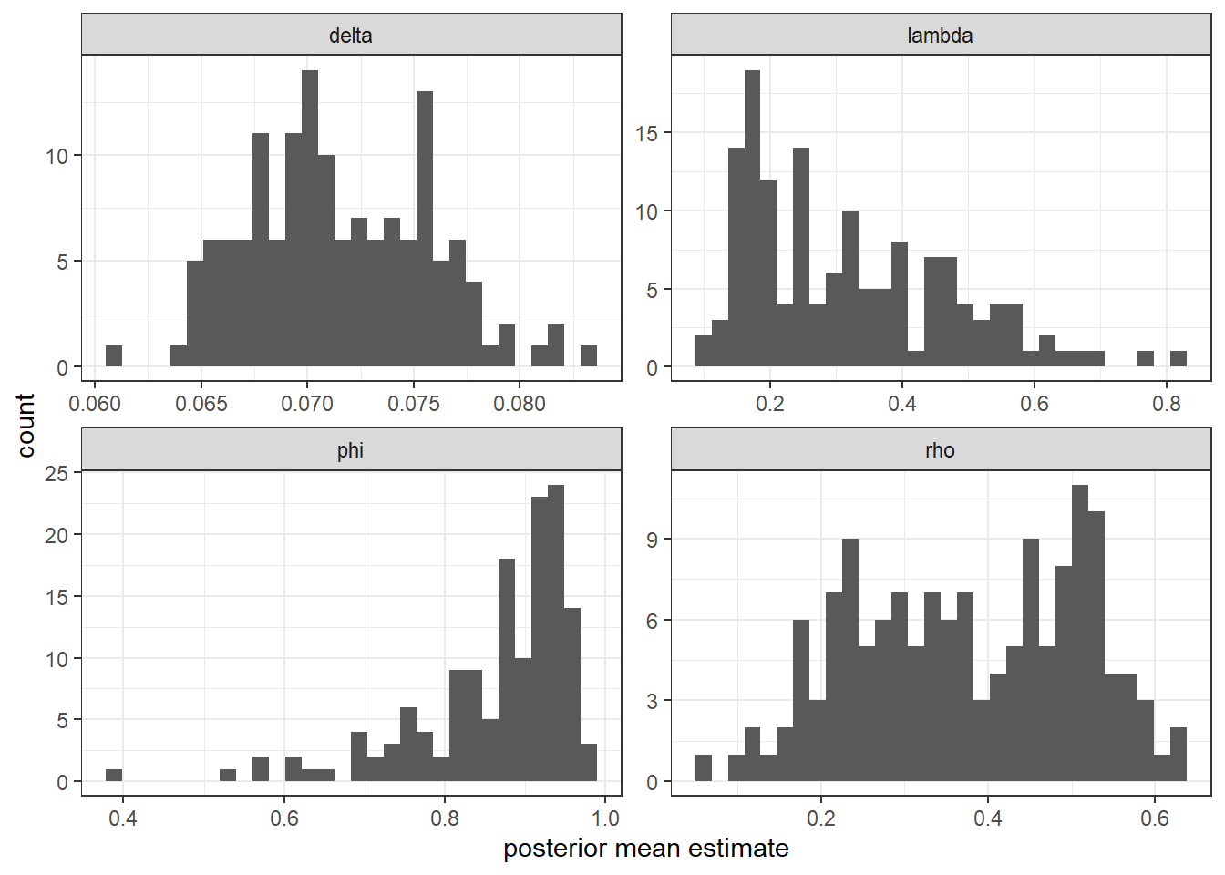
Figure 13.2: Posterior mean estimates of individual-level parameters.
One way I like to visualize the individual-level parameters is to show the empirical cumulative density function (ecdf) of the posterior mean overlaid with a Bayesian credible region. This gives you a sense of both scale and precision for these parameters. I do this in Figure 13.3, which overlays the ecdf with 90% Bayesian credible regions. Here we can see that there is very little heterogeneity in \(\delta\), evidenced by the near vertical ecdf and small horizontal scale on this panel. Coupled with the narrow credible regions only covering values close to zero, we can be fairly certain for most participants that reinforcement learning (\(\delta = 0\)) is a much better approximation of behavior than is weighted fictitious play (\(\delta = 1\)). \(\rho\) appears to be the parameter that we learn the least about, as many of its credible regions cover a wide range of the unit interval. On the other hand, \(\phi\) is estimated reasonably accurately.
(
  ggplot(
    IndParamsLong |>
      group_by(id,parameter) |>
      summarize(mean = mean(value),
                p05 = quantile(value,probs = 0.05),
                p95 = quantile(value,probs = 0.95)
                ) |>
      ungroup() |>
      group_by(parameter) |>
      arrange(mean) |>
      mutate(ecdf = (1:n())/n())

    ,
    aes(x=mean,y=ecdf,xmin=p05,xmax=p95)
  )
  #+geom_point(size = 0.2)
  +stat_ecdf()
  +geom_errorbar(alpha = 0.1)
  +theme_bw()
  +facet_wrap(~parameter,scales="free")
  +xlab("posterior mean estimate")
  +ylab("empirical cumulative density")
)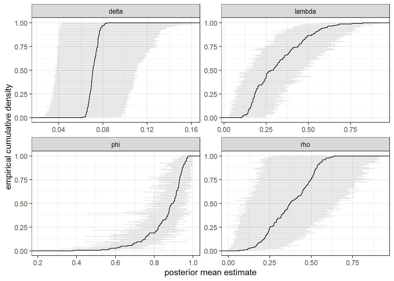
Figure 13.3: Posterior estimates of individual-level parameters. Empirical cumulative density of posterior means overlayed with 90% Bayesian credible regions.
13.5 Some code used to estimate the models
Here is the R code used to load the data and estimate the models.
13.5.1 Loading the data
library(tidyverse)
library(rstan)
rstan_options(auto_write = TRUE)
options(mc.cores = parallel::detectCores())

D<- "Data/CFH2010TASP/TASP-12Sess.csv" |>
  read.csv() |>
  select(session,period,subject,stableID,hi_payID,group,direction) |>
  mutate(id = paste(session,subject) |> as.factor() |> as.numeric()) |>
  # direction is coded as 0,1,2,3. If I code it as 1,2,3,4 then I can reference
  # the payoff matrix
  mutate(direction = direction+1) |>
  arrange(id,period) |>
  group_by(period,session,group) |>
  mutate(direction_other = sum(direction)-direction) |>
  ungroup() |>
  # Link this to the payoff matrices below
  mutate(gameCode = stableID+1,
         hi_payID = hi_payID+1
         )


#-----------------------------------------
# Wrangle data into a Stan-friendly format
#-----------------------------------------

# Here I am going to make everything TxN arrays, or in some cases TxNx4

nPeriods<-length(D$period |> unique())
nParticipants<-length(D$id |> unique())

# PROBLEM: There was a tornado during session 4, and so these participants
# only played 70 rounds, not 80. To see this, note this
D |> group_by(session) |> summarize(maxPeriod=max(period))

ID <-array(0,dim = c(nPeriods,nParticipants))
PERIOD <-array(0,dim = c(nPeriods,nParticipants))
DIRECTION<-array(1,dim = c(nPeriods,nParticipants))
DIRECTION_OTHER<-array(1,dim = c(nPeriods,nParticipants))
GAME_CODE<-array(1,dim = c(nPeriods,nParticipants))
HIPAY<-array(1,dim = c(nPeriods,nParticipants))

for (ii in 1:length(unique(D$id))) {
  d<-D |> filter(id==ii)

  ID[1:dim(d)[1],ii]<-d$id
  PERIOD[1:dim(d)[1],ii]<-d$period
  DIRECTION[1:dim(d)[1],ii]<-d$direction
  DIRECTION_OTHER[1:dim(d)[1],ii]<-d$direction_other
  GAME_CODE[,ii]<-d$gameCode[1]
  HIPAY[1:dim(d)[1],ii]<-d$hi_payID
}

USEDATA<-1*(ID!=0)


payoffs<-list(
  #Unstable
  rbind(
    c(90,0,120,20),
    c(120,90,0,20),
    c(0,120,90,20),
    c(90,90,90,0)
  ),
  #Stable
  rbind(
    c(60,0,150,20),
    c(150,60,0,20),
    c(0,150,60,20),
    c(90,90,90,0)
  )
)


nActions<-dim(payoffs[[1]])[1]

PAYOFFS<-array(NA,dim=c(2,4,4))

PAYOFFS[1,,]<-payoffs[[1]]
PAYOFFS[2,,]<-payoffs[[2]]


gameCode<-(D |> filter(period==1))$gameCode


PI<-array(0,dim=c(nPeriods,nParticipants,nActions))
I<-array(0,dim=c(nPeriods,nParticipants,nActions))
for (ii in 1:nParticipants) {
  U<-payoffs[[gameCode[ii]]]
  for (aa in 1:nActions) {
    PI[,ii,aa]<-U[aa,DIRECTION_OTHER[,ii]]
    I[,ii,aa]<-1*(DIRECTION[,ii]==aa)
  }
}


dStan<-list(
 nPeriods = nPeriods,
 nParticipants = nParticipants,
 nGames = length(payoffs),
 nActions = nActions,

 direction = DIRECTION,

 UseData = USEDATA,
 GameCode = GAME_CODE,

 HiPay = HIPAY,
 payoff_multipliers = c(0.035,0.035),

 payoffs = PAYOFFS,

 PI = PI,
 I  = I,

 prior_phi = c(1,1),
 prior_delta = c(1,1),
 prior_rho = c(1,1),
 prior_lambda = c(1.15,1.76),

 max_payoff = 150*0.035

)

dStan |> saveRDS("Data/CFH2010TASP/CFH2010TASP_dStan.rds")
13.5.2 Estimating the representative agent models
library(tidyverse)
library(rstan)

dStan <- readRDS("Data/CFH2010TASP/CFH2010TASP_dStan.rds")


RAmodel<-stan_model("Code/CFH2010TASP/EWA.stan")

# Model pooling all data
file<-"Code/CFH2010TASP/Estimates_RA_Pooled.rds"
if (!file.exists(file)) {
  print(paste("estimating",file))
  Fit<-sampling(RAmodel,data=dStan,seed=42)
  summary(Fit)$summary |> saveRDS(file=file)
}

# Unstable low payoffs
dd<-dStan$UseData * (dStan$HiPay==1) * (dStan$GameCode==1)
d<-dStan
d$UseData<-dd
file<-"Code/CFH2010TASP/Estimates_RA_UnstableLow.rds"
if (!file.exists(file)) {
  print(paste("estimating",file))
  Fit<-sampling(RAmodel,data=d,seed=42,iter=2000)
  summary(Fit)$summary |> saveRDS(file=file)
}

# Unstable high payoffs
dd<-dStan$UseData * (dStan$HiPay==2) * (dStan$GameCode==1)
d<-dStan
d$UseData<-dd
file<-"Code/CFH2010TASP/Estimates_RA_UnstableHi.rds"
if (!file.exists(file)) {
  print(paste("estimating",file))
  Fit<-sampling(RAmodel,data=d,seed=42)
  summary(Fit)$summary |> saveRDS(file=file)
}

# Stable low payoffs
dd<-dStan$UseData * (dStan$HiPay==1) * (dStan$GameCode==2)
d<-dStan
d$UseData<-dd
file<-"Code/CFH2010TASP/Estimates_RA_StableLow.rds"
if (!file.exists(file)) {
  print(paste("estimating",file))
  Fit<-sampling(RAmodel,data=d,seed=42)
  summary(Fit)$summary |> saveRDS(file=file)
}

# Stable high payoffs
dd<-dStan$UseData * (dStan$HiPay==2) * (dStan$GameCode==2)
d<-dStan
d$UseData<-dd
file<-"Code/CFH2010TASP/Estimates_RA_StableHi.rds"
if (!file.exists(file)) {
  print(paste("estimating",file))
  Fit<-sampling(RAmodel,data=d,seed=42)
  summary(Fit)$summary |> saveRDS(file=file)
}
13.5.3 Estimating the hierarchical model
library(tidyverse)
library(rstan)
  options(mc.cores = parallel::detectCores())
  rstan_options(auto_write = TRUE)


dStan <- readRDS("Data/CFH2010TASP/CFH2010TASP_dStan.rds")


model<-stan_model("Code/CFH2010TASP/EWAhierarchical.stan")

dStan$prior_MU<-list(c(0,0.25),
                     c(0,0.25),
                     c(0,0.25),
                     c(1.15,0.75))

dStan$prior_TAU<-c(0.05,0.05,0.05,0.05)

dStan$prior_OMEGA<-5

dStan$nSimPars<-1000

file<-"Code/CFH2010TASP/Estimates_Hierarchical_Pooled.rds"
if (!file.exists(file)) {
  Fit<-sampling(model,
                data=dStan,
                pars = c("z"),include=FALSE,
                seed=42,
                # The first time running this with the default iter = 2000
                # yielded the "Bulk ESS low" error. This can be remedied with
                # a larger simulation size. Running with these options
                # produced no error
                iter=4000)
  Fit |> saveRDS(file)
}


# I need to work on fixing the divergences here
# So I will hold off on estimating the treatment-specific
# models
References
If you’re playing along at home, these participants are coded as
session = 4.↩︎Another alternative would be to calculate these in the
transformed datablock. For some reason Stan was crashing on me when I did this.↩︎Stan does not have to evaluate derivatives in the
generated quantitiesblock, so things should compute faster here anyway.↩︎The hierarchical model using all of the data produced a Stan fit object that took up about 140MB, and this was after I told it to drop the normalized augmented data. This is certainly not huge by any modern hard drive or RAM requirements, but it is 7% of what Dropbox gives you for free (at the time of writing). ↩︎
But this was still fairly trivial. The kids were having a Nerf battle nearby while I coded, and I was still able to do it :)↩︎
By default, Stan runs 4 chains with 2,000 iterations, but uses 1,000 of these for warm-up. So we are left with 1,000 draws per chain.↩︎
The model using all of the data took a little bit over four hours to run on my laptop with this configuration, so while there is plenty of time to solve a shrine or two while it runs, Hyrule will have to wait a little while longer for its salvation.↩︎
In contrast though, my job market paper (James R. Bland 2019a) estimates a hierarchical model with a similar number of individual-level parameters and participants, but took up something closer to 1GB on my hard drive. This is because the Metropolis-Hastings within Gibbs sampler I implemented for that paper requires many more posterior draws to get the same effective sample size. Hamiltonian Monte Carlo, which is what Stan uses, generally is much more efficient with its draws.↩︎
These can be computed post-estimation from models that use Monte Carlo integration, but they are computed by default when when we use data augmentation.↩︎