16 Computing Quantal Response Equilibrium
Quantal response equilibrium (McKelvey and Palfrey 1995) is an extension of Nash equilibrium that replaces the concept of a best response with a probabilistic best response. That is, instead of choosing an action that is in their best response correspondence, players assign positive probability to all of their actions in a game, and are more likely to take actions that yield greater utility. This extension offers some big advantages over Nash equilibrium when structurally analyzing data from economic experiments. Firstly, the idea of a probabilistic best response is behaviorally plausible. Just as we assume a probabilistic choice rule (like softmax) for individual choice experiments, the same reasons for using this in a game apply: people make mistakes, our model is probably mis-specified, and so on. Secondly, also for the same reasons we use them in individual choice experiments, the probabilistic choice rule permits us to use a likelihood. Otherwise one decision that goes against the prescription of the deterministic component of our model will make the likelihood zero everywhere, and so we cannot simulate a posterior. For games, this is especially a problem when players have a strictly dominated strategy, as these should never be played in equilibrium. Finally, Quantal Response Equilibrium has been shown to organize experimental data a lot better than Nash equilibrium. For example, it models well the “own payoff” effect observed in some games, where Nash equilibrium does not.
Compared to typical structural models for individual choice experiments, the challenges of estimating a Quantal Response Equilibrium model are somewhat unique. Individual choice experiments are sometimes difficult to estimate because it is difficult for our sampler to explore the posterior distribution implied by our likelihood and prior.72 While this problem is by no means ruled out for Quantal Response Equilibrium, its typical computational hurdles come from computing the fixed point condition associated with the equilibrium. I will therefore devote the entirety of this chapter to feasible methods for computing quantal response equilibrium, as this can really make the difference between a model being feasible to estimate or not. As such, this chapter will be more of a computational chapter and less of an estimation chapter. Fear not, I will follow up with a Quantal Response Equilibrium estimation chapter later.
16.1 Overview of quantal response equilibrium
Quantal response equilibrium assumes that players probabilistically best respond to their opponents’ mixed strategies. We model this with a probabilistic best response function, which I will denote as \(q(\lambda,u_{i}(\sigma))\), where \(\lambda>0\) is a choice precision parameter, and \(u_{i,a}(\sigma)\) is the expected utility to player \(i\) of taking action \(a\), given that they are facing mixed strategy profile \(\sigma\). Holding \(\lambda\) constant, \(q_i\) takes a vector of expected utilities \(u_i(\sigma)\), and returns a probability distribution over actions in the player’s choice set, which itself is a vector of probabilities the same size as \(u_i(\sigma)\). Some popular choices of the functional form of \(q\) include the logit or softmax specification:
\[ q_{i,a}(\lambda,u_i(\sigma))=\frac{\exp(\lambda u_{i,a}(\sigma))}{\sum_{b\in A_i}\exp(\lambda u_{i,b}(\sigma))} \]
and the Luce specification:
\[ q_{i,a}(\lambda, u_i(\sigma))=\frac{u_{i,a}(\sigma)^\lambda}{\sum_{b\in A_i} u_{i,b}(\sigma)^\lambda} \]
Note that both of these functions approach best response functions as \(\lambda\to\infty\). At the other end of the parameter space, \(\lambda=0\), players randomize uniformly over their action space.
The “equilibrium” part of Quantal Response Equilibrium comes from assuming that players have correct beliefs about their opponents’ mixed strategies. Mathematically then, the equilibrium condition is:
\[ \sigma_i=q_i(\lambda,u_i(\sigma))\quad \forall i\in \{1, 2, \ldots ,n\} \tag{16.1} \]
That is, every equilibrium mixed strategy \(\sigma_i\) is a probabilistic best response to the equilibrium mixed strategy profile \(\sigma\).
16.2 Computing Quantal Response Equilibrium
Finding a solution to (16.1) can be difficult because it is a fixed point condition: \(\sigma\) appears on both the right- and left-hand side of the equation, and we typically cannot find a closed-form solution. Furthermore, we cannot be guaranteed that it is a contraction, so iterating the equation by first guessing a \(\sigma\), then computing the probabilistic best response profile, and then repeating, will not in general find a solution. A far more reliable way to compute Quantal Response Equilibrium is to use a predictor-corrector algorithm. This algorithm in the context of Quantal Response Equilibrium was developed in Turocy (2005) and Turocy (2010), and is discussed in detail in James R. Bland and Turocy (2026). This algorithm is also implemented in the software package Gambit (McKelvey, McLennan, and Turocy 2022).
16.2.1 Setting up the problem
While it might be more intuitive to think about solving (16.1) exactly as it is written in probability levels, you will likely run into some stability issues if you do. This is because for some games the algorithm will want to jump into “probabilities” that are either less than zero or greater than one. In practice, the problem is much more stable if we first translate (16.1) into log-probability differences. That is, we re-write this equation as:
\[ \begin{aligned} 0=H_{i,a}(\lambda,\sigma)&=\log\sigma_{i,a}-\log\sigma_{i,a+1}-\left(\log q_{i,a}(\lambda,u_i(\sigma))-\log q_{i,a+1}(\lambda,u_i(\sigma))\right)\\ &\forall i\in\{1, 2, \ldots, n\},\ \forall a \in \{1, 2, \ldots ,J_i-1\} \end{aligned} \]
where \(n\) is the number of players and \(J_i\) is the number of actions in player \(i\)’s action space.
This representation is particularly useful, because the log-difference of the probabilistic best responses (the term in the parentheses) for the logit and Luce specifications become:
\[ \begin{aligned} \text{logit: }\quad H_{i,a}(\lambda,\sigma)&=\log\sigma_{i,a}-\log\sigma_{i,a+1}-\lambda\left[u_{i,a}(\sigma)-u_{i,a+1}(\sigma)\right]\\ \text{Luce: }\quad H_{i,a}(\lambda,\sigma)&=\log\sigma_{i,a}-\log\sigma_{i,a+1}-\lambda\left[\log u_{i,a}(\sigma)-\log u_{i,a+1}(\sigma)\right] \end{aligned} \]
respectively. That is, we can cancel out the common denominators.
We then need some adding-up constraints to ensure that the mixed strategies add up to one:
\[ \begin{aligned} 0=H_{i,\Sigma}(\lambda,\sigma)&=\sum_{a=1}^{J_i}\sigma_{i,a}-1,\quad \forall i \in\{1, 2, \ldots ,n\} \end{aligned} \]
Letting \(\rho_{i,a}=\log\sigma_{i,a}\), these constraints become:
\[ \begin{aligned} \text{logit:}\quad H_{i,a}(\lambda,\rho)&=\rho_{i,a}-\rho_{i,a+1}-\lambda\left[u_{i,a}(\exp(\rho))-u_{i,a+1}(\exp(\rho))\right]\\ \text{Luce: }\quad H_{i,a}(\lambda,\rho)&=\rho_{i,a}-\rho_{i,a+1}-\lambda\left[\log u_{i,a}(\exp(\rho))-\log u_{i,a+1}(\exp(\rho))\right]\\ \text{adding up: }\quad H_{i,\Sigma}(\lambda,\rho)&=\sum_{a=1}^{J_i}\exp(\rho_{i,a})-1 \end{aligned} \] where \(\exp(\rho)=\sigma\) is the element-wise exponentiation of \(\rho\).
Stacking all of these together, we have one great big vector of zero conditions defining a quantal response equilibrium:
\[ 0=H(\lambda,\rho)=\begin{pmatrix} H_{1,1} \\ H_{1,2}\\ \vdots \\ H_{1,J_1-1} \\ H_{2,1} \\ \vdots \\ H_{2,J_2-1} \\ \vdots\\ H_{n,J_n-1}\\ H_{1,\Sigma} \\ H_{2,\Sigma}\\\vdots \\ H_{n,\Sigma} \end{pmatrix} \]
16.2.2 A predictor-corrector algorithm
A good way to solve for quantal response equilibrium is to use a predictor corrector algorithm. This algorithm, developed in Turocy (2005) and Turocy (2010), initializes with a known quantal response equilibrium \((\lambda^t,\rho^t)\), then uses information contained in \(H\) find a nearby solution \((\lambda^{t+1},\rho^{t+1})\).
To begin with, we will re-parameterize the problem using \(x\equiv \begin{pmatrix}\rho^\top & \lambda\end{pmatrix}^\top\). This is because the algorithm does not really make a distinction between the parameters \(\rho\) and \(\lambda\).
A quantal response equilibrium \((\lambda,\rho)\) can therefore be characterized as a solution to:
\[ H(x)=0 \]
where \(H(x)\) is a \({\sum_{i=1}^n}J_i \times 1\) vector. Furthermore, since the solutions of \(H(x)=0\) form a smooth, differentiable curve in the \(\rho-\lambda\) space, we can trace out this curve using information contained in \(H\). Specifically, we will use the jacobian of \(H\) to make a first-order approximation of the curve. We will then use the zero condition to correct any errors that come from this approximation.
Following the initialization, the algorithm applies two distinct steps:
First, in the predictor step, the algorithm makes a first-order approximation of the path continues from point \(x^t\) to point \(x^{t+1}\). This approximation is found using the total derivative of \(H\):
\[ \begin{aligned} \frac{\partial H(x)}{\partial x^\top}\Delta x\approx0 \end{aligned} \]
There are many solutions to this equation.73 What we really need from this is a direction to move. To do this, we can take a “fat” QR decomposition of the transpose of the jacobian \(\frac{\partial H(x)}{\partial x^\top}\). The final column of the \(Q\) that comes out of this gives us the direction we want, and has magnitude one. Therefore the predictor step is:
\[ \begin{aligned} x^{t+1}&=x^t+h\omega Q_{,-1}(x_t) \end{aligned} \] where:
- \(Q_{,-1}(x_t)\) is the final column of the \(Q\) component of the “fat” QR decomposition of \(\left[\frac{\partial H(x_t)}{\partial x^\top}\right]^\top\). We can compute the fat decomposition of matrix \(A\) in R using
qr(A) |> qr.Q(complete=TRUE).74 - \(\omega\in\{-1,1\}\) ensures that we are moving in the right direction along the curve, and not back-tracking. For example, if we are looking to trace out the curve for increasing \(\lambda\), then \(\omega\) will have the same sign as the last element in \(Q_{,-1}(x_t)\), which corresponds to \(\lambda\).
- \(h>0\) is a tuning parameter specifying the step length. Recall that the magnitude of \(Q_{,-1}(x_t)\) has a magnitude of 1, so \(h\) is the step length.
As noted in Turocy (2005), while it may be feasible to solve for quantal response equilibrium using only predictor steps, which are a form of numerical integration, this ignores some information that we have about quantal response equilibrium: it is characterized by a solution to a set of equations.75 Therefore, we can also exploit these equations to correct any errors that may have made their way into the system equations because the predictor step is only an approximation of the change in \(x\). Specifically, the following corrector step moves \(x\) in the direction that gets \(H(x^{t+1})\) closer to zero:
\[ x^{t+1}=x^t-\left(\frac{\partial H(x^t)}{\partial x^\top}\right)^+ H(x^t) \]
where \(A^+\) is the Moore-Penrose inverse of \(A\). We can compute this inverse in R using ginv(A), which comes in the MASS library. We iterate on the corrector step until it has reached our desired level of accuracy.
16.2.3 Initial conditions
So once we have one solution to \(H(\lambda,\rho)=0\), we can trace out many other solutions. Great! But how do we initialize the problem? That is, we are doing this because we want to compute quantal response equilibrium, but we need to know one in order to start the algorithm. Fortunately, there are a couple of natural starting places. The simplest to start with is at the centroid: \(\lambda=0\), \(\sigma_{i,a}=1/J_i\) will always be a quantal response equilibrium. That is, when choice precision is zero, they payoffs of the game don’t matter, and uniform randomization is the equilibrium strategy profile. The path \(\{(\lambda,\rho): H(\lambda,\rho)=0,\lambda\geq 0\}\) starting at the centroid and \(\lambda=0\) is called the “principal branch”, and is often used to select an equilibrium when multiple are present.
Other places to consider starting might be ones close to a Nash equilibrium. This is because quantal response equilibrium will nest every Nash equilibrium when \(\lambda\to\infty\). Therefore starting with \(\lambda^0 =\) something very large, and \(\rho^0=\log\sigma^\text{Nash}\), then tracing out the branch from there might also be useful. Of course, computing Nash equilibrium can be difficult, too, so this starting point may not be computationally feasible in some games.
16.2.4 Algorithm tuning
The predictor-corrector algorithm described above allows us to choose two tuning parameters in order to (hopefully) improve the algorithm’s performance.
- For the predictor step, we can choose the step size \(h\), which pins down how large is \(\|x^{t+1}-x^t\|\)
- For the corrector step, we can choose the stopping rule, which defines how accurate is “accurate enough” for our solution to \(H(0)=0\).
A good solution to this is to choose a desired level of accuracy for the corrector step, and then use the number of iterations needed in the corrector step to adjust the predictor step’s step length \(h\). Broadly speaking, if the corrector step requires a lot of iteration, then the previous predictor step jumped too far, and so we should reduce \(h\) for the next step. On the other hand if only a few iterations are needed for the corrector step, then we could have jumped further using the predictor step without too much loss of accuracy, so increasing \(h\) in this case is warranted.
16.3 The predictor-corrector algorithm in R
Here is my implementation of the predictor-corrector algorithm in R. It is unashamedly translated from Ted Turocy’s Python code, which accompanies our paper James R. Bland and Turocy (2026).
# Needed for the Moore-Penrose inverse
library(MASS)

PC<-function(
             # A named list comprising of functions H, Hlambda, and Hrho
             Hlist,
             # Total number of actions in the game
             nActions,
             # range of lambda to compute QRE for. First element is the starting point. Second element can be above or below this
             lambda_span, # c(lambda0,lambda_end)
             # Starting poring for log probabilities
             x0, # rho0
             # first step size
             first_step,
             # Minimum step size
             min_step,
             # Maximum deceleration of step size
             max_decel,
             # Maimum number of iterations for corrector step
             maxiter,
             # Tolerance for corrector step (a step size)
             tol
) {


  # unpack the list of functions Hlist

  H<-Hlist[["H"]]
  Hlambda<-Hlist[["Hlambda"]]
  Hrho<-Hlist[["Hrho"]]

  jac<-function(x) {
    cbind(Hrho(x[nActions+1],x[1:nActions]),Hlambda(x[nActions+1],x[1:nActions]))
  }
  # Maximum distance to curve
    max_dist <- 0.4
    # Maximum contraction rate in corrector
    max_contr <- 0.6
    # Perturbation to avoid cancellation in calculating contraction rate
    eta <- 0.1

    # Initial conditions
    x<-c(x0,lambda_span[1])
    QRE<-rbind(c(),x)


    # The last column of Q in the QR decomposition is the tangent vector
    t <- (qr(jac(x) |> t())  |> qr.Q(complete=TRUE))[,nActions+1]

    h<-first_step

    # Set orientation of curve, so we are tracing into the interior of `t_span`
    omega<-sign(t[nActions+1])*sign(lambda_span[2]-lambda_span[1])


   while ((x[nActions+1]>=min(lambda_span)) & (x[nActions+1]<=max(lambda_span))) {
   accept <-TRUE

     if (abs(h)<= min_step) {
       # Stepsize below minimum tolerance; terminate.
       success <-FALSE
       print(paste("Stepsize",abs(h),"less than minimum",min_step))
       break
     }

     # Predictor step
     u<-x + h*omega*t
     q<-qr(jac(u) |> t())  |> qr.Q(complete=TRUE)

     disto <- 0
     decel <- 1/max_decel # deceleration factor

     for (it in 1:maxiter) {
       y<-H(u[nActions+1],u[1:nActions])


       # change in rho proposed by Newton step
       # This is the step we'd use if we kept lambda constant
       #drho <- -solve(Hrho(u[nActions+1],u[1:nActions]),y)
       drho<- - ginv(jac(u)) %*% y
       dist<-(drho^2) |> sqrt() |> sum()


       if (dist >= max_dist) {
         print(paste("Proposed distance",dist,"exceeds max_dist =",max_dist))
         accept<-FALSE
         break
       }

       decel<-max(c(decel,sqrt(dist/max_dist)*max_decel))

       if (it>1) {
         contr<- dist/(disto +tol*eta)
         if (contr > max_contr) {
           print(paste("Maximum contraction rate exceeded"))
           accept<-FALSE
           break
         }
         decel <-max(c(decel,sqrt(contr/max_contr)*max_decel))
       }
       if (dist < tol) {

         # Success! update and break out of iteration
         break
       }
       disto<-dist

       # if we have got to this point, then:
       #  1. The Newton step has not proposed a too-large change
       #  2. The contraction rate has not been exceeded
       #  3. The proposed Newton step is not so small that we have effectively
       #    found a solution
       # Therefore, we update rho

       u<-u+drho


       if (it==maxiter) {
         # We have run out of iterations. Terminate
         print(paste("Maximum number of iterations",maxiter,"reached"))
       }

     } ## END OF CORRECTOR STEP

       if (!accept) {
         # Step was not accepted; take a smaller step and try again
         h<-h/max_decel
       }

       # Standard steplength adaptation
       h<-abs(h/min(c(decel,max_decel)))

       # Update with outcome of successful PC step
       if (sum(t*q[,nActions+1])<0) {
         # The orientation of the curve as determined by the QR
         # decomposition has changed.
         #
         # The original Allgower-Georg QR decomposition implementation
         # ensures the sign of the tangent is stable; when it is stable
         # the curve orientation switching is a sign of a bifurcation.
         omega<- -omega
         #print("sign of omega flipped")
       }


       x<-u
       t<-q[,nActions+1]

       #print(c(exp(x[1:nActions]),x[nActions+1]))


        QRE<-rbind(QRE,x |> as.vector())
        #print(c(exp(x[1:nActions]),x[nActions+1]) |> t())


   }
  QRE


}

# Save the function so I can use it in later chapters if needed

PC |> saveRDS("Code/QRE1/PCalgorithm.rds")
16.4 Some example games
16.4.1 Generalized matching pennies (Ochs 1995)
To begin with, I will show you the logit quantal response equilibrium for a generalized matching pennies game. Generalized matching pennies games are a good place to start due to their simplicity: there is only one path that we have to follow, which is the principal branch connecting the centroid \((\rho^0,0)\) to the unique Nash equilibrium. Therefore we can be sure to trace out all quantal response equilibria by starting at the centroid. The game, studied in Ochs (1995), is shows in Table 16.1. This game is also used as an example in McKelvey and Palfrey (1995).
| L | R | |
|---|---|---|
| U | 4, 0 | 0, 1 |
| D | 0, 1 | 1, 0 |
Here is some working constructing the function \(H\) and finding its derivatives:
\[ \begin{aligned} H(\lambda,\rho)&=\begin{pmatrix} \rho_U-\rho_D -\lambda(4\exp(\rho_L)-1\exp(\rho_R))\\ \rho_L-\rho_R-\lambda(-1\exp(\rho_U)+1\exp(\rho_D))\\ \exp(\rho_U)+\exp(\rho_D)-1\\ \exp(\rho_L)+\exp(\rho_R)-1 \end{pmatrix} \\~\\ \frac{\partial H(\lambda,\rho)}{\partial \lambda} &=\begin{pmatrix} -(4\exp(\rho_L)-1\exp(\rho_R))\\ -(-1\exp(\rho_U)+1\exp(\rho_D))\\ 0\\0 \end{pmatrix} \\ ~ \\ \frac{\partial H(\lambda,\rho)}{\partial \rho^\top}&= \begin{bmatrix} 1 & -1 & -4\lambda\exp(\rho_L) & +1\lambda \exp(\rho_R)\\ 1\lambda\exp(\rho_U) & -1\lambda\exp(\rho_D) & 1 & -1\\ \exp(\rho_U) & \exp(\rho_D) & 0 & 0\\ 0 & 0 & \exp(\rho_L) & \exp(\rho_R) \end{bmatrix} \end{aligned} \]
And here is how we pass this information to the solver function I wrote above:
GMP<-list(
  # Function defining QRE conditions
  H = function(lambda,rho) {
    rbind(
      rho[1]-rho[2]-lambda*(4*exp(rho[3])-1*exp(rho[4])),
      rho[3]-rho[4]-lambda*(-1*exp(rho[1])+1*exp(rho[2])),
      exp(rho[1])+exp(rho[2])-1,
      exp(rho[3])+exp(rho[4])-1
    )
  },
  # derivative with respect to lambda
  Hlambda = function(lambda,rho) {
    rbind(
      -(4*exp(rho[3])-1*exp(rho[4])),
      -(-1*exp(rho[1])+1*exp(rho[2])),
      0,
      0
    )
  },
  # derivative with respect to rho
  Hrho = function(lambda,rho) {
    rbind(
      c(1,-1,-4*lambda*exp(rho[3]),1*lambda*exp(rho[4])),
      c(1*lambda*exp(rho[1]),-1*lambda*exp(rho[2]),1,-1),
      c(exp(rho[1]),exp(rho[2]),0,0),
      c(0,0,exp(rho[3]),exp(rho[4]))
    )
  }
)

     QRE<-   PC(GMP,
             4, # total number of actions
             c(0,100), # c(lambda0,lambda_end)
             rep(log(0.5),4), # rho0
             0.1, # first step size
             1e-4,# minimum step size
             1.1, # max deceleration
             1000, # maximum number of iterations
             1e-4 # tolerance
        )

QRE<-cbind(exp(QRE[,1:4]),QRE[,5])
colnames(QRE)<-c("U","D","L","R","lambda")

QRE<-QRE |> data.frame()

(
  ggplot(QRE,aes(x=U,y=L))
  +geom_path(linewidth=1)
  +theme_bw()
  +coord_fixed(xlim=c(0,1),ylim=c(0,1))
)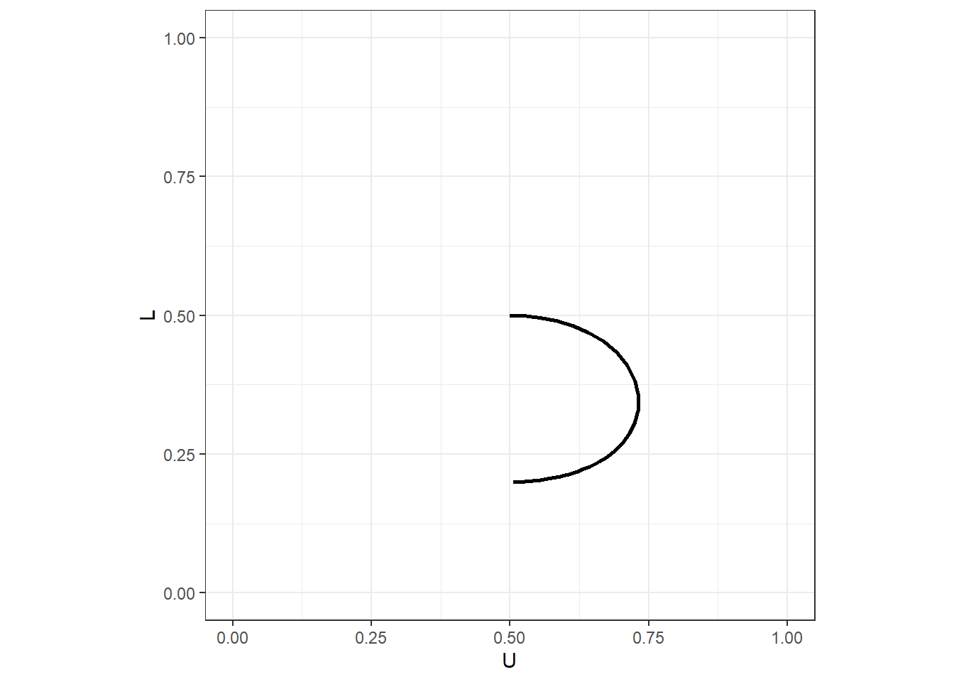
Figure 16.1: Locus of logit quantal response equilibrium probabilities for a generalized matching pennies game.
Figure @(fig:QRE1GMPlocus) shows the logit quantal response equilibrium locus. This is the set of mixed strategy profiles that are a quantal response equilibrium. While this kind of plot obfuscates the choice precision parametrer \(\lambda\), I really like to show a QRE this way, as it very clearly shows the kind of predictions that it can make.76
However to visualize the curves that the predictor-corrector algorithm is actually tracing out, you need to include \(\lambda\). This is shown in Figure 16.2. Note that I have included \(\lambda\) on a log scale. For this plot this transformation ensures that all of the interesting stuff isn’t squished up into the first 10% of horizontal coordinates.
(
  ggplot(QRE,aes(x=lambda))
  +geom_path(aes(y=U,linetype="U"),linewidth=1)
  +geom_path(aes(y=L,linetype="L"),linewidth=1)
  +scale_x_continuous(trans="log10")
  +theme_bw()
  +xlab(expression(lambda))
  +ylab("Mixed strategy")
  +scale_linetype_discrete(name="")
)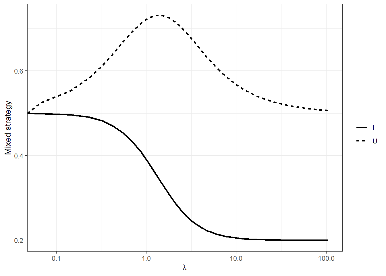
Figure 16.2: Logit quantal response equilibrium of generalized matching pennies game as a function of choice precision \(\lambda\)
16.4.2 Stag hunt
Table 16.2 shows a stag hunt game, which is a coordination game with three Nash equilibria: \((U,L)\), \((D,R)\), and \(\sigma_U=\sigma_L=a/4\). This should get us a bit worried about computing quantal response equilibrium, because we will not find all of the paths if we just start at the centroid. To begin with, let’s set up the system of equations, and see what happens when we start at the centroid. Here I am going to take advantage of the symmetry of the game, noting that I can set \(\sigma_U=\sigma_L\) without loss of generality.
| L | R | |
|---|---|---|
| U | 4, 4 | 0, a |
| D | a, 0 | a, a |
\[ \begin{aligned} H(\lambda,\rho) &= \begin{pmatrix} \rho_U-\rho_D-\lambda(4\exp(\rho_U)-a)\\ \exp(\rho_U)+\exp(\rho_D)-1 \end{pmatrix} \\ \frac{\partial H(\lambda,\rho)}{\partial \rho^\top} &=\begin{bmatrix} 1-4\lambda\exp(\rho_U) & -1\\ \exp(\rho_U) & \exp(\rho_D) \end{bmatrix} \\ \frac{\partial H(\lambda,\rho)}{\partial \lambda} &=\begin{pmatrix} -(4\exp(\rho_U)-a)\\ 0 \end{pmatrix} \end{aligned} \]
StagHunt<-function(a) {
  list(
  H = function(lambda,rho) {
    rbind(
      rho[1]-rho[2]-lambda*(4*exp(rho[1])-a),
      exp(rho[1])+exp(rho[2])-1
    )
  }
  ,
  Hrho = function(lambda,rho) {
    rbind(
      c(1-4*lambda*exp(rho[1]),-1),
      c(exp(rho[1]),exp(rho[2]))
    )
  }
  ,
  Hlambda = function(lambda,rho) {
    rbind(
      -(4*exp(rho[1])-a),
      0
    )
  }
)
}

a<-1

QRE1<-   PC(StagHunt(a),
             2, # total number of actions
           c(0,10),
           rep(log(0.5),2), # rho0
             0.03, # first step size
             1e-4,# minimum step size
             1.1, # max deceleration
             1000, # maximum number of iterations
             1e-4 # tolerance
        )

QRE1[,1:2]<-exp(QRE1[,1:2])

QRE1<-QRE1 |> data.frame()
colnames(QRE1)<-c("U","D","lambda")

(
  ggplot(QRE1,aes(x=lambda,y=U))
  +geom_path(linewidth=1)
  +theme_bw()
  +scale_x_continuous(trans="log10")
  +xlab(expression(lambda))
  +geom_hline(yintercept=c(0,1,a/4),linetype="dashed")
)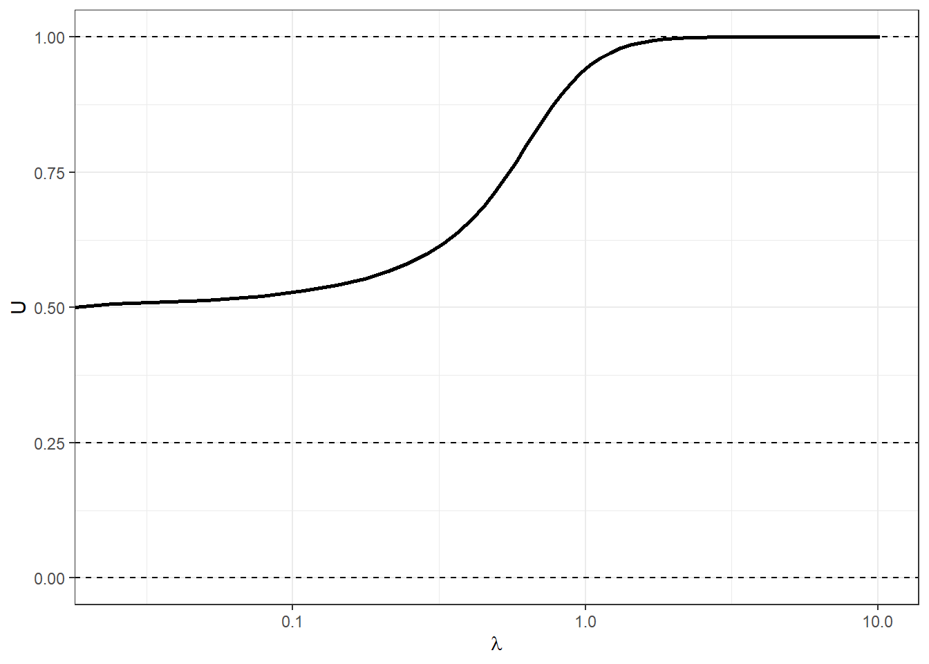
Figure 16.3: The principal branch of the logit quantal response equilibrium of the stag hunt game with \(a=1\).
Tracing out the principal branch of the logit QRE is done in exactly the same way as we did it for the asymmetric matching pennies games. This branch is shown in Figure 16.3 for \(a=1\). However note that we have only approach one of the three Nash equilibria, which are shown with horizontal dashed lines. In order to trace out the other parts of the quantal response equilibrium, we need to give the predictor-corrector algorithm different starting points. Let’s do this and add them to the principal branch:
# Starting close to the mixed strategy Nash equilibrium

QRE2<-   PC(StagHunt(a),
             2, # total number of actions
           c(20,0),
           c(log(a/4),log(1-a/4)), # rho0
             0.001, # first step size
             1e-4,# minimum step size
             1.01, # max deceleration
             1000, # maximum number of iterations
             1e-4 # tolerance
        )

QRE2[,1:2]<-exp(QRE2[,1:2])

QRE2<-QRE2 |> data.frame()
colnames(QRE2)<-c("U","D","lambda")

## Joining them together

QRE<-rbind(
  QRE1 |> mutate(branch = "Principal"),
  QRE2 |> mutate(branch = "Other")
)

(
  ggplot(QRE,aes(x=lambda,y=U,color=branch))
  +geom_path(linewidth=1)
  +theme_bw()
  +scale_x_continuous(trans="log10")
  +xlab(expression(lambda))
  +geom_hline(yintercept=c(0,1,a/4),linetype="dashed")
)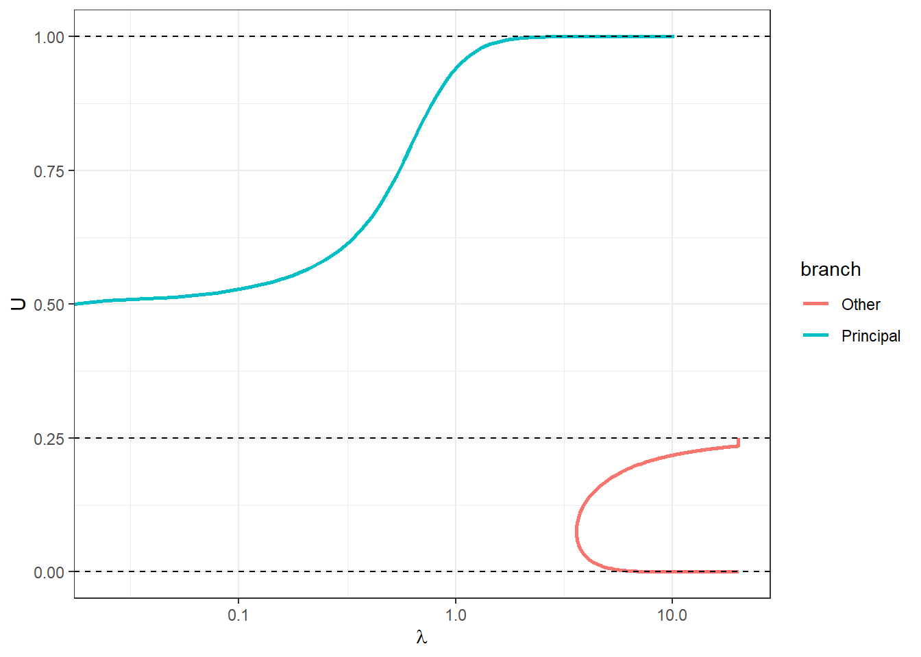
Figure 16.4: Logit quantal response equilibrium branches for the stag hunt game with \(a=1\).
The principal branch is shown alongside the other branch in Figure 16.4. Note with the above code that I had to tweak some of the tuning parameters: max_deceleration is much smaller, which means that the step size will change more slowly. What is also apparent from this Figure is that we can get turning points in \(\lambda\). This can be seen in the “Other” branch (red curve). We therefore cannot always parameterize these curves as a function of \(\lambda\).
An interesting knife-edge case for this game is when \(a=2\). Here the principal branch is constant at \(\sigma_U=0.5\), and hence is always equal to the mixed strategy Nash equilibrium. In this case, we get a bifurcation, and the two pure-strategy Nash equilibria are connected by a branch. Therefore, the only way to compute the non-principal branch is to start really close to one of the pure-strategy Nash equilibria. For this case, suppose we start close to the Nash equilibrium where \(\sigma_U=0\). This means that the expected utility of playing \(U\) will be approximately zero (for large but finite \(\lambda\)), and the expected utility of playing \(D\) will be \(a=2\). Therefore the approximate quantal response equilibrium mixed strategy for large \(\lambda\) will be:
\[ \sigma_U(\lambda)\approx(1+\exp(-\lambda(0-2)))^{-1} \]
a<-2


QRE1<-   PC(StagHunt(a),
             2, # total number of actions
           c(0,10),
           rep(log(0.5),2), # rho0
             0.03, # first step size
             1e-4,# minimum step size
             1.1, # max deceleration
             1000, # maximum number of iterations
             1e-4 # tolerance
        )

QRE1[,1:2]<-exp(QRE1[,1:2])
QRE1<-QRE1 |> data.frame()
colnames(QRE1)<-c("U","D","lambda")

lambdaStart<-10

QRE2<-   PC(StagHunt(a),
             2, # total number of actions
           c(lambdaStart,0),
           c(-log(1+exp(2*lambdaStart)),-log(1+exp(-2*lambdaStart))), # rho0
             0.03, # first step size
             1e-4,# minimum step size
             1.01, # max deceleration
             1000, # maximum number of iterations
             1e-4 # tolerance
        )

QRE2[,1:2]<-exp(QRE2[,1:2])
QRE2<-QRE2 |> data.frame()
colnames(QRE2)<-c("U","D","lambda")

QRE<-rbind(
  QRE1 |> mutate(branch = "Principal"),
  QRE2 |> mutate(branch = "Other")
)

(
  ggplot(QRE,aes(x=lambda,y=U,color=branch))
  +geom_path(linewidth=1)
  +theme_bw()
  +scale_x_continuous(trans="log10")
  +xlab(expression(lambda))
  +geom_hline(yintercept=c(0,1,a/4),linetype="dashed")
)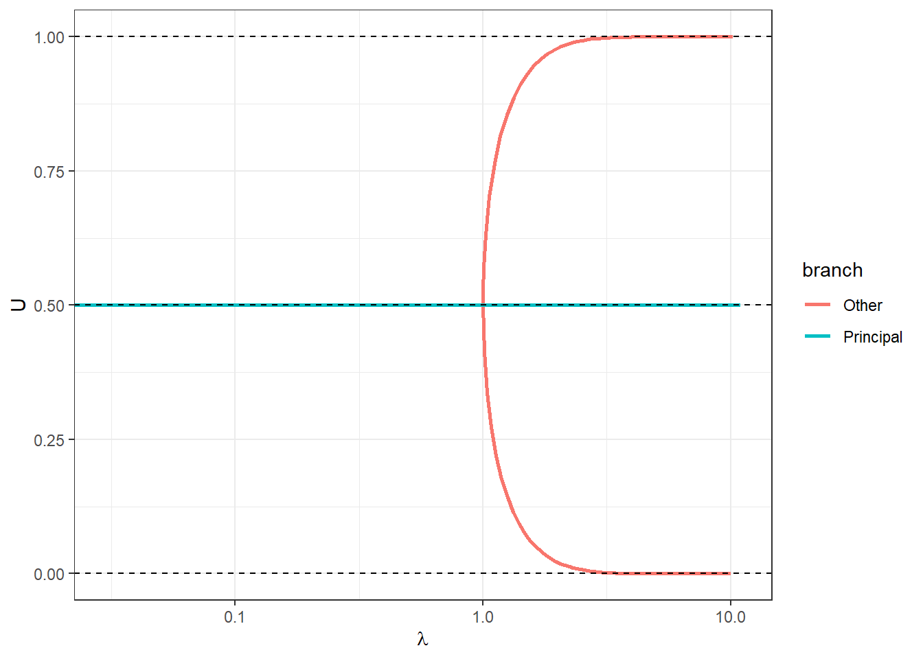
Figure 16.5: Logit quantal response equilibrium branches for the stag hunt game with \(a=2\).
16.4.3 \(n\)-player Volunteer’s Dilemma imposing symmetric strategies
In their experimental analysis of the Volunteer’s Dilemma (Diekmann 1985), Goeree, Holt, and Smith (2017) analyze the data through the lens of the symmetric quantal response equilibrium, which assumes that all players volunteer with the same probability.77 The Volunteer’s dilemma is an \(n\geq 2\) person game, and is summarized in Table 16.3. Each player either volunteers (\(V\)) at a private cost of \(c\), or does not volunteer \(D\) at no cost. If at least one player volunteers, then all players earn \(V>c\), and if no player volunteers, all earn \(L<V-c\).
| At least one other player volunteers | Nobody else volunteers | |
|---|---|---|
| Volunteer | V-c | V-c |
| Don’t volunteer | V | L |
The symmetry assumption here greatly simplifies the equilibrium predictions. For example, in Nash equilibrium, it rules out everything except for the symmetric mixed strategy Nash equilibrium. Similarly for quantal response equilibrium, we are left just with the equilibria where everybody volunteers with probability \(\sigma_V(\lambda)\). In working out the payoff differences needed to compute quantal response equilibrium, it is useful to have an expression for the probability that none of the \(n-1\) opponents volunteer:
\[ \begin{aligned} p(\text{nobody else volunteers})&=\sigma_N^{n-1}\\ &=\exp(\rho_N)^{n-1}\\ &=\exp((n-1)\rho_N) \\ p(\text{at least one other player volunteers})&=1-\exp((n-1)\rho_N) \end{aligned} \]
These can then be used to construct \(H(\rho,\lambda)\) and its derivatives as follows:
\[ \begin{aligned} H(\lambda,\rho) &=\begin{pmatrix} \rho_V - \rho_N -\lambda(V-c-V(1-\exp((n-1)\rho_N))-L\exp((n-1)\rho_N)))\\ \exp(\rho_V)+\exp(\rho_N)-1 \end{pmatrix}\\ \frac{\partial H(\lambda,\rho)}{\partial \rho^\top} &=\begin{bmatrix} 1 & -1-\lambda(n-1)\exp((n-1)\rho_N)\left(V-L\right)\\ 1 & 1 \end{bmatrix} \\ \frac{\partial H(\rho,\lambda)}{\partial \lambda} &=\begin{pmatrix} -(V-c-V(1-\exp((n-1)\rho_N))-L\exp((n-1)\rho_N)))\\ 0 \end{pmatrix} \end{aligned} \]
Here are these functions coded in R:
VolunteersDilemma<-function(n,V,c,L) {
  list(
    H = function(lambda,rho) {
      rbind(
        rho[1]-rho[2]-lambda*(
          V-c-V*(1-exp((n-1)*rho[2]))-L*exp((n-1)*rho[2])
        ),
        exp(rho[1])+exp(rho[2])-1
      )
    }
    ,
    Hrho = function(lambda,rho) {
      rbind(c(1, -1-lambda*(n-1)*exp((n-1)*rho[2])*(V-L)),
            c(1, 1)
      )
    }
    ,
    Hlambda = function(lambda,rho) {
      rbind(
        -( V-c-V*(1-exp((n-1)*rho[2]))-L*exp((n-1)*rho[2])),
        0
      )
    }
  )
}
And now we can solve this for a few values of the group size \(n\) (here I hold \(V=1\), \(c=0.1\), and \(L=0.2\) constant):
QRE<-data.frame()

for (nn in 2:6) {

  qre<-PC(VolunteersDilemma(nn,1,0.1,0.2),
               2, # total number of actions
             c(0,1000),
             rep(log(0.5),2), # rho0
               0.03, # first step size
               1e-4,# minimum step size
               1.1, # max deceleration
               1000, # maximum number of iterations
               1e-4 # tolerance
          )

  qre[,1:2]<-exp(qre[,1:2])
  colnames(qre)<-c("V","D","lambda")

  QRE<-rbind(
    QRE,
    qre |>
      data.frame() |>
      mutate(`group size` = nn)
  )

}

(
  ggplot(QRE,aes(x=lambda,y=V,color=as.factor(`group size`)))
  +geom_path(linewidth=1)
  +theme_bw()
  +scale_x_continuous(trans="log10")
  +xlab(expression(lambda))
  +ylab("Probability of volunteering")
  +scale_color_discrete(name="group size")
  +ylim(c(0,1))

)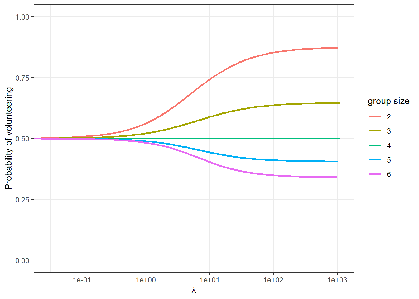
Figure 16.6: The symmetric quantal response equilubrium paths for the \(n\)-player Volunteer’s Dilemma with \(V=1\), \(c=0.1\) and \(L=0.2\)
References
Loosely speaking, this is a similar problem to it being hard to maximize the likelihood in these applications.↩︎
For example, if \(\Delta x\) is a solution to this equations, \(c\Delta x\) for \(c\in\mathbb R\) is also a solution.↩︎
This was a major time suck for me in converting Ted Turocy’s Python code into R, because the default options in each language are different. By default, Python computes the fat decomposition, but R does not. ↩︎
That is, the predictor steps are equivalent if we are solving \(H(x)=0\), or \(H(x)=\) any other vector of constants. In the predictor step, we explicitly take advantage of this being a zero condition.↩︎
You can see a lot of plots like this one in James R. Bland and Turocy (2026) and James R. Bland (2023a).↩︎
They then extend the model to investigate several motivations for heterogeneneous volunteering probabilities, which I might get to later.↩︎