5 Representative agent and participant-specific models

Our participants are not homogeneous. Therefore representative agent models do not get us very far, both as economic models, and as econometric models. For economic models, this is because choices do not aggregate unless preferences meet some very strict criteria. Econometric models motivated from these economic models will inherit these problems, and create their own. In particular, we should be worried about heterogeneity bias, which occurs when we assume that a parameter is homogeneous across participants, when it is in fact heterogeneous. For example Wilcox (2006) shows that conclusions about the type of learning that participants are doing in a game will be biased in favor of one model (reinforcement learning) if heterogeneity is not addressed in the econometric model.

While I therefore avoid pooled representative agent models for most of my work, they do provide us with a useful stepping stone in taking an economic model through the process of becoming a probabilistic econometric model. Estimating a representative agent model, even if we do not take it too seriously, is a useful proof-of-concept before advancing further into the depths of the hierarchical structure that our data probably deserves. This is because the representative agent model will likely identify certain coding or computational issues that are specific to your problem. For example in Bland (2022) I spent a lot of time honing my pooled Quantal Response Equilibrium model before moving on to the hierarchical and off-equilibrium specifications. This first established for me that it was in fact feasible to estimate a Quantal Response Equilibrium model at all in Stan. If it hadn’t been, I would have discovered this much earlier in the research process than had I tried to do the hierarchical, off-equilibrium with risk-aversion model first. In the process I was able to identify the bits of the code that were slowing things down, and work out more speedy solutions to computing Quantal Response Equilibrium in a much simpler environment. Furthermore, as you will see in some later chapters of this book, almost all of the work that follows once you have a representative agent model to extend it to a hierarchical or mixture model is quite mechanical: it will look the same irrespective of the specific model you are taking to the data. As such, once you get the hang of these more complicated specifications, I suspect that you will actually spend more time thinking about the parts of your code that would also be in the representative agent model.

Representative agent models are also useful if all we want are participant-specific estimates. When all we are using are data from one participant, the representative agent and the participant are the same person. Instead, the “representative agent” assumption is probably better called a “stable preferences” assumption, where we are assuming that the participant’s utility function remains the same for the entire experiment. In this chapter, I will therefore present you with a guide to estimating participant-specific models.

5.1 Participant-specific models

5.1.1 Example data and economic model

In this section, I will use data from the modified dictator games in Bruhin, Fehr, and Schunk (2019). In this part of the experiment, 174 participants made 78 pairwise choices over allocations of money between themself and another participant. The 78 pairwise allocations, and the choices of the first participant to show up in the data, can be seen in Figure 5.1. Here you can see these choices described by a line connecting the two allocations. There is a dot at the allocation chosen by the first participant. In this Figure you can see that each participant is presented with choices where they always earn less than the other person (top-left corner), when they always earn more than the other person (bottom-right corner), and when the two allocations span over both of these regions (in the middle of the plot).

library(tidyverse)

d1<-(read.csv("Data/BFS2019_choices_exp1.csv")
     |> mutate(experiment=1)
)
d2<-(read.csv("Data/BFS2019_choices_exp2.csv")
     |> mutate(experiment=2)    
)
D<-(rbind(d1,d2)
     # Just use the dictator game data
     |> filter(dg==1)  
     |> mutate(
       self_alloc = ifelse(choice_x==1,self_x,self_y),
       other_alloc = ifelse(choice_x==1,other_x,other_y)
     )
)

(
  ggplot(
    D |> filter(sid==102010050706),
    
  )
  +geom_segment(aes(x=self_x,y=other_x,xend=self_y,yend=other_y))
  +geom_point(aes(x=self_alloc,y=other_alloc))
  +theme_bw()
  +xlab("Own payoff")+ylab("Other's payoff")
  +geom_abline(slope=1,intercept=0,linetype="dashed")
  +coord_fixed()
)

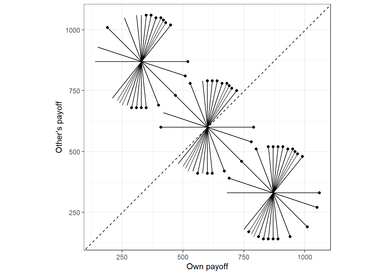
The 78 pairwise choices over allocations of money. Each pariwise choice is denoted by the endpoints of a line. The decisions of the first participant are shown as dots at the chosen endpoint.

Figure 5.1: The 78 pairwise choices over allocations of money. Each pariwise choice is denoted by the endpoints of a line. The decisions of the first participant are shown as dots at the chosen endpoint.

Bruhin, Fehr, and Schunk (2019) estimate the parameters in the Fehr and Schmidt (1999) model, which assumes that the decision-maker’s utility over allocations of money is linear in their own earnings, and the earnings of the other person, but there is a change in the marginal utility of money depending on whether the other person is earning less or more than the decision-maker. Here is the Fehr and Schmidt (1999) model (written just for two people, which is all we have here):

\[ U(\pi_1,\pi_2;\alpha,\beta)= \pi_1-\alpha\max\{\pi_2-\pi_1,0\}-\beta\max\{\pi_1-\pi_2,0\} \]

Where $\pi_1$ is the decision-maker’s earnings, $\pi_2$ is the other person’s earnings, and $\alpha$ and $\beta$ are the parameters of the model. Fehr and Schmidt (1999) further impose the parameter restrictions of $\beta\in[0,1]$ and $\alpha>\beta$, which make it a model of inequality aversion: all else held equal, the decision-maker prefers equal allocations of money. Restricting $\beta<1$ means that the decision-maker would not be willing to burn money to equalize earnings. As these are parameter restrictions that are testable, I will instead estimate the models without these restrictions, and then comment on how empirically relevant these parameter restrictions seem to be. This is also how Bruhin, Fehr, and Schunk (2019) approaches the problem.

Other than the restrictions initially imposed by Fehr and Schmidt (1999), it is also meaningful to divide the $\alpha$-$\beta$ space into four regions based on the signs of these parameters. These regions tell us qualitatively the kind of preferences that the parameters imply:

$\alpha>0$ and $\beta>0$: the participant is inequality-averse. Holding their own income equal, they prefer outcomes where the other person earns the same as them.
$\alpha<0$ and $\beta<0$: the participant is inequality-loving. Holding their own income equal, they prefer to have the other person earning a lot more or a lot less than them.
$\alpha<0$ and $\beta>0$: the participant is efficiency-loving. Holding their own income equal, they prefer the other person to earn more.
$\alpha>0$ and $\beta<0$: The participant is efficiency-averse or competitive. Holding their own income equal, the prefer the other person to earn less.

5.1.2 Going to the probabilistic model

Since we have a deterministic model specified above, we need to modify it so that it makes probabilistic predictions. As we have binary choice, it does not make sense to estimate a “optimal choice plus error” model. Therefore I will use the utility-based model of probabilistic choice discussed in the previous chapter: logit choice. This is also the model used in the maximum likelihood specification of Bruhin, Fehr, and Schunk (2019). In the data, each allocation is coded as “Choice X” and “Choice Y”, and the binary variable identifying which allocation is chosen is equal to one if and only if X is chosen. Therefore, we can parameterize the logit choice model as follows:

\[ \Pr\left(X_{i,t}=1\mid \alpha_i,\beta_i,\lambda_i\right) =\Lambda\left(\lambda\left(U(\pi_{1,t}^X,\pi_{2,t}^X;\alpha,\beta)-U(\pi_{1,t}^Y,\pi_{2,t}^Y;\alpha,\beta)\right)\right) \]

where $\Lambda(x)=1/(1+\exp(-x))$ is the inverse logit function.

We could also do this by specifying a distribution:

\[ X_{i,t}\sim \mathrm{Bernoulli}\left(\Lambda\left(\lambda\left(U(\pi_{1,t}^X,\pi_{2,t}^X;\alpha,\beta)-U(\pi_{1,t}^Y,\pi_{2,t}^Y;\alpha,\beta)\right)\right)\right) \]

Therefore we have three parameters to estimate: $\alpha$ and $\beta$, the parameters in the original economic model, and logit choice precision $\lambda$, which we need to make the model probabilistic.

5.1.3 A short side quest into canned estimation techniques

Before moving on, it is very important to note a practical implication of the Fehr and Schmidt (1999) model with logit choice: it is a logit model. As in, it is a logit model like you might estimate in Stata or R!. This is an immensely useful realization that could speed up your analysis if you were OK with estimating this model with pre-packaged estimation routines. Specifically, with a few transforms of the data, you can estimate $\lambda$, and (linear transforms of) $\alpha$, and $\beta$ using a standard logit. To see this, note that we can transform the data as follows:

\[ \begin{aligned} d^X&=\max\{\pi_2-\pi_1,0\},\quad a^X=\max\{\pi_1-\pi_2\} \end{aligned} \]

and similarly for allocation $Y$, we can then write the model as:

\[ \begin{aligned} \Pr(X_{i,t}\mid \alpha_i,\beta_i,\lambda_i) &=\Lambda\left(\lambda\left(\pi_{1,t}^X-\alpha_id_{t}^X-\beta_id_t^X-\pi_{1,t}^Y+\alpha_id_{t}^Y+\beta_id_t^Y\right)\right)\\ &=\Lambda\left(\lambda(\pi^X_{i,t}-\pi^Y_{i,t})+\lambda\alpha_i(d^Y_t-d^X_t)+\lambda\beta_i(a^Y_t-a^X_t)\right) \end{aligned} \]

which is a logit model without an intercept, and so we can estimate the model as follows (here I am just doing it for the first participant):

library(stargazer)
D<-(
  D
  |> rowwise()
  |> mutate(dX = max(c(0,other_x-self_x)),
            dY = max(c(0,other_y-self_y)),
            aX = max(c(0,self_x-other_x)),
            aY = max(c(0,self_y-other_y))
            )
  |> ungroup()
  |> mutate(x1 = self_x-self_y,
            x2 = dY-dX,
            x3 = aY-aX)
)
model<-glm(data=D|> filter(sid==102010050706),
           formula=choice_x~x1+x2+x3-1,
           family=binomial(link="logit")) 
stargazer(model,type="html",digits=6)


	Dependent variable:

	choice_x

x1	0.008173^***
	(0.001845)

x2	0.000443
	(0.001339)

x3	0.001269
	(0.001277)


Observations	78
Log Likelihood	-38.115470
Akaike Inf. Crit.	82.230940

Note:	p<0.1; p<0.05; p<0.01

So here we have $\hat\lambda=0.0081731$. We haven’t directly estimated $\alpha$ and $\beta$. Instead, we have estimated $\lambda\alpha$ and $\lambda\beta$, so we need to divide by $\hat\lambda$ to get $\hat\alpha=0.0541735$, and $\hat\beta=0.1552275$.

5.1.4 Assigning priors

Up to this point, I have not talked much about priors. This stops here! Our priors are the information we give our econometric model as experts (yes, you’re one of them) about the economic model.

Let’s start with the choice precision parameter $\lambda$. For me, this is always the most difficult to assign, because it does not have a great economic interpretation. Sure, larger values mean more precise choices, but you really don’t have any idea about scale until you look at some predictions implied by it. Let’s calibrate this prior to a reasonable distribution based on what it implies about the choices of a self-regarding participant. That is, when we set the other paranmeters $\alpha=\beta=0$, what do the probabilistic predictions of our model look like as we change $\lambda$. To do this, I will first get a smaller dataset together of all the unique payoff differences faced by a selfish decision-maker:

d<-(D
    |> mutate(absDiff = abs(self_x-self_y))
    |> dplyr::select(absDiff)
    |> unique()
    )

d |> as.vector() |> print()

## $absDiff
##  [1] 140 200 380 240 120  80  40 280 180   0 160 360

It looks like we have twelve of them. Let’s plot the probability of choosing the action with the greatest payoff against $\lambda$. Since $\lambda$ (kind-of) happens on a log scale, it is helpful to have this in a log scale:

lambdaCheck<-(
  expand.grid(lambda = 1/(1-seq(0.0001,0.6,length=1001))-1,
              absDiff = d$absDiff)
  |> mutate(
    PrOptimal = 1/(1+exp(-lambda*absDiff))
  )
)
(
  ggplot(data=lambdaCheck,aes(x=lambda,y=PrOptimal,group=absDiff))
  +geom_path()
  +theme_bw()
  +scale_x_continuous(trans="log10")
  +xlab("\u03bb")+ylab("Probability of choosing the action with the higher payoff")
)

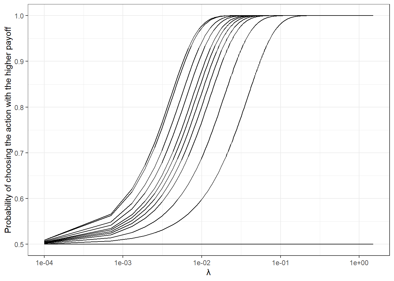
$Probability of choosing the optimal action for selfish decison-makers as a function of choice precision $\lambda$. Each curve shows the model's prediction for a different payoff difference from the experiment.$

Figure 5.2: Probability of choosing the optimal action for selfish decison-makers as a function of choice precision $\lambda$. Each curve shows the model’s prediction for a different payoff difference from the experiment.

It looks to me like most of the interesting stuff happens at $\lambda<0.1$. Since $\lambda$ must be positive, I will use a log-normal prior, which gives me two parameters to play with, the location and scale:¹⁶

\[ \log\lambda\sim N(m_\lambda,s_\lambda^2) \] I will calibrate this prior so that the 95th percentile of $\lambda$ is 0.1, and the 5th percentile of $\lambda$ is 0.0001. The system of equations to solve this is:

\[ \begin{aligned} \log 0.1&=m_\lambda+1.64s_\lambda\\ \log0.0001&=m_\lambda-1.64s_\lambda\\ \log(0.1)-\log(0.0001)&=2\times1.64s_\lambda\\ s_\lambda&=\frac{\log(0.1)-\log(0.0001)}{2\times 1.64}\approx 2.11\\ m_\lambda &=\log0.1-1.64\times2.11\approx-5.76 \end{aligned} \]

That leaves us with assigning priors to $\alpha$ and $\beta$. I will lump these together and use the same prior for both parameters. I think this simplification of the problem is OK because we can interpret both of these as marginal utilities. Here I note that if either parameter is greater than one in absolute value, then the participant will respond very strongly to inequality (or efficiency, or something else, depending on their signs). Let’s place 75% of the prior probability mass of both parameters in the range $(-1,1)$, which means that our full prior distribution is:

\[ \begin{aligned} \alpha&\sim N(0,0.67^2)\\ \beta &\sim N(0,0.67^2)\\ \log\lambda&\sim N(-5.76,2.11^2) \end{aligned} \]

5.1.5 Estimating the model for one participant

Here is the Stan program I wrote to estimate this model. Note that you could have generated the transformed data before passing it to Stan and got the same results. I just wanted to have the program take the data as close as possible to how it is on the journal website.


data {
  int<lower=0> n; // number of observations
  vector[n] self_x; // payoff to self with allocation x
  vector[n] other_x; // payoff to other with allocation x
  vector[n] self_y; // payoff to self with allocation y
  vector[n] other_y; // payoff to other with allocation y
  int choice_x[n]; // =1 iff allocation x is chosen
  
  real prior_lambda[2];
  real prior_alpha[2];
  real prior_beta[2];
}

transformed data {
  vector[n] dX; // disadvantageous inequality at allocation x
  vector[n] dY; // disadvantageous inequality at allocation y
  vector[n] aX; // advantageous inequality at allocation X
  vector[n] aY; // advantageous inequality at allocation X
  
  dX = fmax(0,other_x-self_x);
  dY = fmax(0,other_y-self_y);
  aX = fmax(0,self_x-other_x);
  aY = fmax(0,self_y-other_y);
}
parameters {
  real alpha;
  real beta;
  real<lower=0> lambda;
}
model {
  
  vector[n] Ux; // utility of allocation x
  vector[n] Uy; // utility of allocation y
  
  Ux = self_x-alpha*dX-beta*aX;
  Uy = self_y-alpha*dY-beta*aY;
  
  // likelihood
  choice_x ~ bernoulli_logit(lambda*(Ux-Uy));
  
  // priors
  alpha~normal(prior_alpha[1],prior_alpha[2]);
  beta ~normal(prior_beta[1],prior_beta[2]);
  lambda ~ lognormal(prior_lambda[1],prior_lambda[2]);
  
}

Before moving on, I want to draw your attention to the vectorization used in this program. Specifically, since I have the data variables self_x, dX, and aX stored as vectors, and the model’s parameters alpha and beta are just real numbers (i.e. scalars), I can calculate the entire utility of Option X (and likewise for Option Y) in one line without looping over all observations. That is, the following two methods for calculating the utility of Option X will produce the same result:

// the vectorized method
Ux = self_x-alpha*dX-beta*aX;

// a for loop
for (ii in 1:n) {
  Ux[ii] = self_x[ii]-alpha*dX[ii]-beta*aX[ii];
}

However the second method will take longer. This is because Stan is geared towards vectorized calculations and matrix operations. The second option may seem more intuitive to you (it does to me), but I encourage you to see the matrix and vectorize things where you can. It’s not going to same much time for this model, but as we start estimating more complicated models every bit of speed-up helps.

Now, let’s estimate the model for the first participant

library(rstan)
rstan_options(auto_write = TRUE)
options(mc.cores = parallel::detectCores())

file<-"RepAgentModels/RepAgentModels_BFS2019"

# only run if I haven't estimated it yet
if (!file.exists(paste0("Outputs/",file,"_subj1.rds"))) {
  ii<-102010050706
  d<-D |> filter(sid==ii)
  dStan<-list(
    n=dim(d)[1],
    self_x=d$self_x,
    other_x=d$other_x,
    self_y=d$self_y,
    other_y=d$other_y,
    choice_x=d$choice_x,
    
    # Stan (and R for that matter) deal with standard deviations, 
    # not variances for a normal distribution
    prior_lambda = c(-5.76,2.11),
    prior_alpha=c(0,0.67),
    prior_beta = c(0,0.67)
  )
  Fit<-stan(paste0("Code/",file,".stan"),
            data=dStan,
            seed=42)
  saveRDS(Fit,paste0("Outputs/",file,"_subj1.rds"))
}

Fit<-readRDS(paste0("Outputs/",file,"_subj1.rds"))

rstan::summary(Fit)$summary %>% knitr::kable(caption="Estimates from the first participant in @BFS2019")

Table 5.1: Estimates from the first participant in Bruhin, Fehr, and Schunk (2019)
	mean	se_mean	sd	2.5%	25%	50%	75%	97.5%	n_eff	Rhat
alpha	0.0889337	0.0038723	0.1932936	-0.2584474	-0.0372583	0.0778896	0.2045905	0.5094519	2491.683	1.001793
beta	0.1377641	0.0035096	0.1816480	-0.2167278	0.0241048	0.1406289	0.2529966	0.4902746	2678.910	1.001272
lambda	0.0072245	0.0000376	0.0018702	0.0038158	0.0058960	0.0071869	0.0084521	0.0110631	2471.567	1.000313
lp__	-40.8879873	0.0382728	1.4314119	-44.5129399	-41.5399276	-40.5390461	-39.8432989	-39.2968401	1398.780	1.000426

Table 5.1 shows the estimates summary, which is not too dissimilar from the point estimates from the logit above (there is lots of uncertainty in both kinds of estimate, so take into consideration the standard errors as well).

sim<-tibble(alpha = rstan::extract(Fit)$alpha,beta=rstan::extract(Fit)$beta)
(
  ggplot(sim,
         aes(x=alpha,y=beta))
  +geom_point(size=0.3,alpha=0.1)
  +geom_vline(xintercept=0,linetype="dashed")
  +geom_hline(yintercept=0,linetype="dashed")
  +theme_bw()
  +xlab(expression(alpha))+ylab(expression(beta))
)

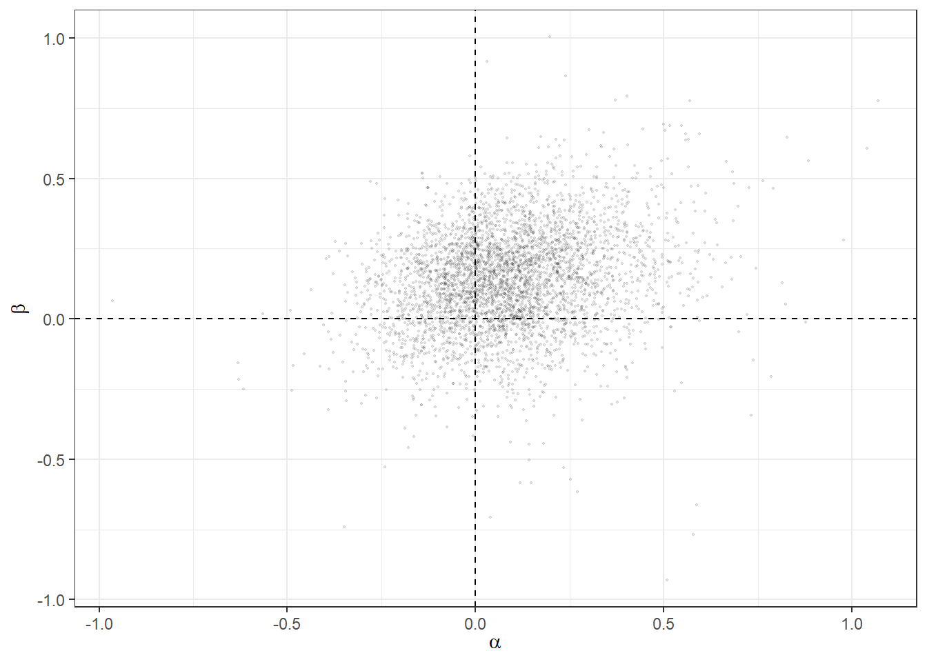
Posterior draws for the first participant of @BFS2019.

Figure 5.3: Posterior draws for the first participant of Bruhin, Fehr, and Schunk (2019).

Figure 5.3 shows the 4,000 posterior draws from the posterior distribution of $\alpha$ and $\beta$. We can use these draws to work out a posterior probability that the parameters lies in each quadrant of this plot, which can help us assign a posterior probability to this participant having the parameter restrictions imposed by Fehr and Schmidt (1999), which are:

$\alpha>0$ and $\beta>0$, so the participant is averse to inequality,
$\alpha>\beta$, so the participant dislikes being behind (aversion to disadvantageous inequality) more than being ahead, and
$\beta\in(0,1)$, so the participant would not be willing to burn money in order to equalize payoffs

To compute the probability that all of these are true, we simply compute the fraction of posterior draws that satisfy these conditions:

sim |> summarize(
  FS1999 = mean(
    alpha>0 & beta>0 & alpha>beta & beta<1
  )
)

## # A tibble: 1 × 1
##   FS1999
##    <dbl>
## 1  0.233

Since I centered the prior distribution on zero for both of these parameters, 23% is not too different from 25%, the prior probability that these conditions are met. Therefore I would not get too excited about this probability. Furthermore, since we have 4,000 posterior draws, the prior standard deviation of this probability is at least:¹⁷

\[ \sqrt{\frac{0.25\times0.75}{4000}}\approx 0.007 \]

So getting 4,000 draws from the prior that implied that this probability was 23% would not be too unlikely. All of this is to say, we actually don’t learn much about whether this parameter restriction is relevant for this participant. We actually do resolve quite a bit of parameter uncertainty, though. For example, Figure 5.4 shows both the prior and posterior distributions of $\alpha$. We have actually learned quite a bit from these 78 choices, but it is more that we have rules out large values of $\alpha$, rather than ruled out everything on one side of zero. As such, the uncertainty in whether or not $\alpha>0$ is largely unchanged.

(
  ggplot()
  +geom_density(data=sim,aes(x=alpha,linetype="posterior"))
  +geom_path(data=tibble(alpha=seq(-2,2,length=1000)) |> mutate(den=dnorm(alpha,mean=0,sd=0.67)),aes(x=alpha,y=den,linetype="prior"))
  +theme_bw()
  +xlab(expression(alpha))+ylab("density")
)

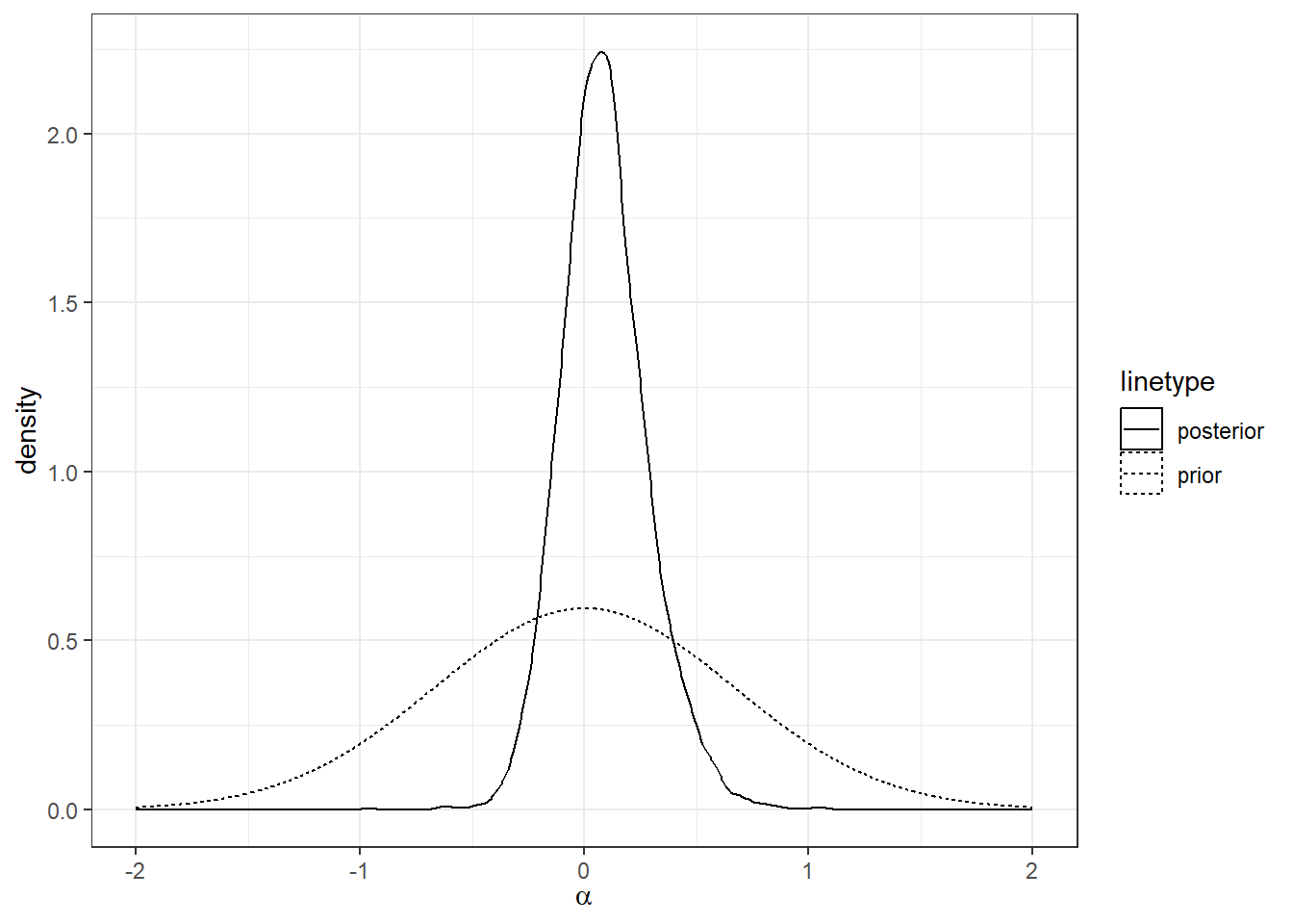
$Prior and posterior distributions of parameter $\alpha$ for the first particiapnt in @BFS2019.$

Figure 5.4: Prior and posterior distributions of parameter $\alpha$ for the first particiapnt in Bruhin, Fehr, and Schunk (2019).

5.1.6 Estimating the model for all participants

Of course, once we have a model that we can estimate for one participant, we can also use it with the others. So here we go:¹⁸

if (!file.exists(paste0("Outputs/",file,"_ALL.rds"))) {
  
  # create an empty dataset to dump the posterior draws into
  ESTIMATES<-tibble()
  
  for (ii in (D$sid |> unique())) {
    print(ii)
    d<-D|> filter(sid==ii)
    
    dStan<-list(
    n=dim(d)[1],
    self_x=d$self_x,
    other_x=d$other_x,
    self_y=d$self_y,
    other_y=d$other_y,
    choice_x=d$choice_x,
    
    # Stan (and R for that matter) deal with standard deviations, 
    # not variances for a normal distribution
    prior_lambda = c(-5.76,2.11),
    prior_alpha=c(0,0.67),
    prior_beta = c(0,0.67)
  )
  Fit<-stan(paste0("Code/",file,".stan"),
            data=dStan,
            seed=42,
            # Here I am running into a few "divergent transitions"
            # errors. One of the solutions to this is to increase 
            # the "adapt_delta" control parameter
            control=list(adapt_delta=0.999)
            )
  
  tmp<-tibble(lambda = extract(Fit)$lambda,
              alpha  = extract(Fit)$alpha,
              beta   = extract(Fit)$beta,
              sid    = ii
              )
  ESTIMATES<-rbind(ESTIMATES,tmp)
    
  }
  
  saveRDS(ESTIMATES,paste0("Outputs/",file,"_ALL.rds"))
}

So that’s all very well and good, but what do we do with all of these estimates? We don’t have the time to look at a summary output table for each one of them individually, so things are best summarized in pictures. What I will do here is wrangle the posterior draws into posterior means and 95% Bayesian credible regions,¹⁹ and also the probability that the Fehr and Schmidt (1999) parameter restriction holds.

ESTIMATES<-readRDS(paste0("Outputs/",file,"_ALL.rds"))
  
# a summary of estimates that I could have got from summary(Fit)$summary
EstSum<-(
  ESTIMATES
  |> pivot_longer(cols=c(lambda,alpha,beta),values_to="value")
  |> group_by(sid,name)
  |> summarize(
    mean = mean(value),
    p025 = quantile(value,probs=0.025),
    p975 = quantile(value,probs=0.975)
  )
)

# Probability that the FS restriction holds
ProbFS1999<-(
  ESTIMATES
  |> group_by(sid)
  |> summarize(PrFS = mean(
    alpha>0 & beta>0 & alpha>beta & beta<1
    )
  )
)

First, let’s look at the probability that the Fehr and Schmidt (1999) restriction holds. As before this is just a matter of computing the fraction of times the posterior draws land in the right region. The empirical cumulative density of these posterior probabilities is shown in Figure 5.5.²⁰ Here we can see a large accumulation of posterior probabilities near zero. About 60% of participants have so few posterior draws of $\alpha$ and $\beta$ in the region implied by the Fehr and Schmidt (1999) restriction that we cannot distinguish between zero and the actual posterior probability. As such, there are in fact very few participants whose parameters are likely to conform to the Fehr and Schmidt (1999) restriction.

(  
  ggplot(ProbFS1999,aes(x=PrFS))
  +stat_ecdf()
  +theme_bw()
  +xlab("Posterior probability that the FS restriction on \n parameters holds")
  +ylab("empirical cumulative density")
)

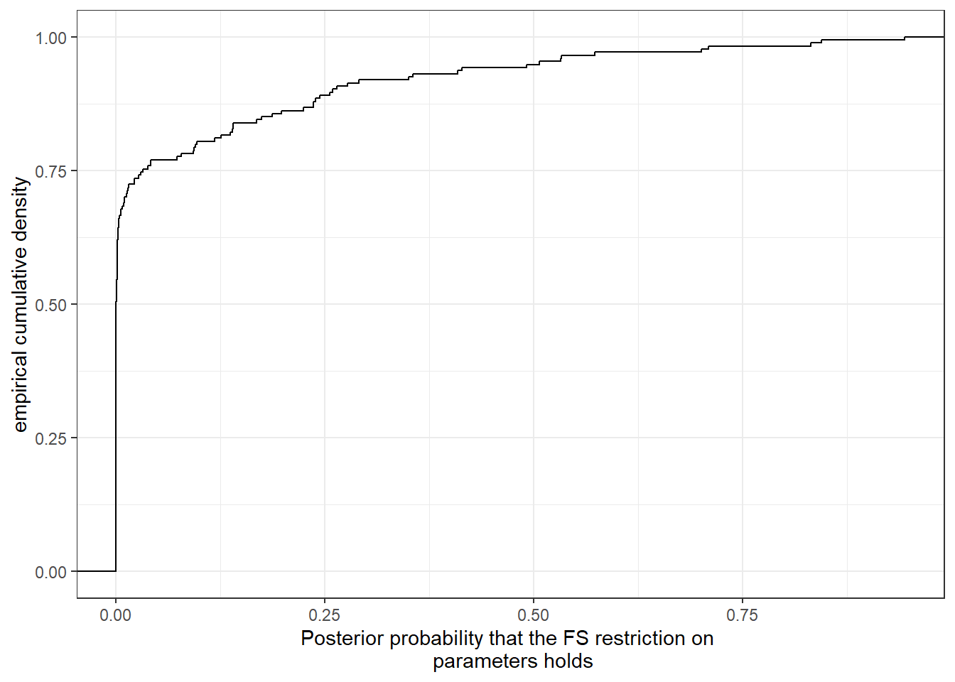
Posterior probability that the @FS1999 restrictions hold for each participant.

Figure 5.5: Posterior probability that the Fehr and Schmidt (1999) restrictions hold for each participant.

Now let’s try to visualize the joint distribution of participants’ parameters. It can get really messy in these plots if you try to show a credible region around the point estimates, so here I will just plot the posterior means. These are shown in Figure 5.6. The majority of these point estimates fall in the efficiency-loving region ($\alpha<0$, $\beta>0$), and within this most estimates have $\beta>|\alpha|$, meaning that these participants care more about increasing the other person’s earnings when the other person is earning less than themself. The majority of parameters are also less than one in absolute value, meaning that they place more weight on their own earnings than they do on the earnings of others. The obvious exception to this is for three competitive and inequality averse participants with $\alpha>1$. For these participants, their marginal utility of own wealth is less than their marginal utility of the other person’s wealth when the other person is earning more. There are no particiapnts whose posterior mean estimates are in the inequality loving quadrant of this plot.

regions<-tibble(
  alpha = c(1,-0.25,-0.25,1),
  beta = c(0.5,-0.5,0.8,-0.5),
  label = c("inequality averse",
            "inequality loving",
            "efficiency loving",
            "competitive"
            )
)

pltInd<-(  
  ggplot(
    data = (ESTIMATES |> group_by(sid)
                      |> summarize(alpha = mean(alpha),
                                   beta = mean(beta),
                                   lambda = mean(lambda))
            
            ),
    aes(x=alpha,y=beta,color=log10(lambda))
  )
  +geom_point()
  +geom_text(data=regions,aes(x=alpha,y=beta,label=label),color="black")
  +theme_bw()
  +xlab(expression(alpha))+ylab(expression(beta))
  +geom_hline(yintercept=0,linetype="dashed")
  +geom_vline(xintercept=0,linetype="dashed")
  #+geom_abline(slope=c(-1,1),intercept=0,linetype="dotted")
)
pltInd |> print()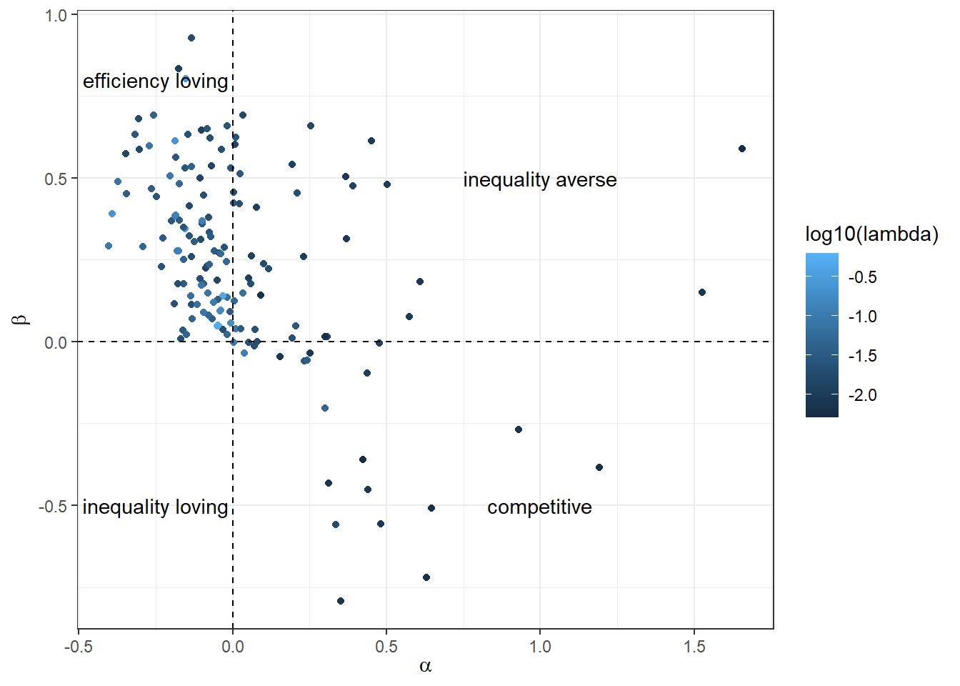

Posterior mean estimates for @FS1999 model using data from @BFS2019. Dashed lines show boundaries for the classification of types of preferences.

Figure 5.6: Posterior mean estimates for Fehr and Schmidt (1999) model using data from Bruhin, Fehr, and Schunk (2019). Dashed lines show boundaries for the classification of types of preferences.

Finally, if we want a deeper dive into the parameters individually, we can plot the empirical cumulative density function of the posterior means, overlaying them with their 95% Bayesian credible regions to show how precise the estimates are. This is done in Figure 5.7. I like these plots both for individual estimation and for hierarchical models because they show us a lot of information about the between-participant heterogeneity in the parameter estimates, as well as giving us an idea about how precise our estimates are. Here we can see that there is substantial heterogeneity both in the posterior mean estimates (seen in the empirical cumulative density functions), as well as in the precision of the estimates (seen in the error bars).

(  
  ggplot(data=(EstSum 
               |> filter(name!="lambda")
               |> group_by(name) 
               |> mutate(rank=rank(mean)/length(mean))
               )
  )
  +facet_wrap(~name,scales="free")
  +stat_ecdf(aes(x=mean))
  +geom_errorbar(aes(y=rank,xmin=p025,xmax=p975),alpha=0.5)
  +theme_bw()
  +ylab("empirical cumulative density")
  +xlab("posterior estimate")
)

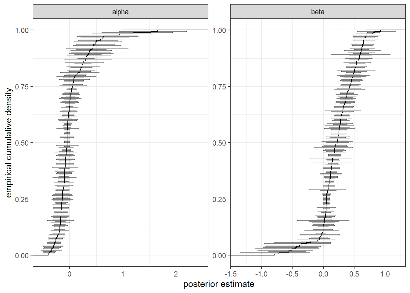
$Empirical cumulative density functions of posterior mean estimates for $\alpha$ and $\beta$. Error bars show 95% Bayesain credible regions for the parameter.$

Figure 5.7: Empirical cumulative density functions of posterior mean estimates for $\alpha$ and $\beta$. Error bars show 95% Bayesain credible regions for the parameter.

5.1.7 But we could be learning more!

Hopefully the above analysis is leaving you somewhat disappointed. OK, we have estimated some individual-specific parameters, but they are still quite imprecise. From a practical perspective, why even bother doing Bayesian estimation for this when there is a pre-packaged Frequentist logit function in every statistical package?²¹ Perhaps more annoyingly (for me at least), we haven’t yet got a way of estimating a distribution of parameters and then commenting on the population of these preferences in any meaningful way. We might have been able to do some scatter plots of our parameters and made qualitative comments about any patterns or clusters that we might see, but what we really need is a way to organize the data of the whole experiment, rather than just for one participant at a time. This will be the focus especially of the next chapter (hierarchical models), and many others to follow will build on this. For the remainder of this chapter, though, we will continue to learn a bit more about representative agent models.

5.2 Actual representative agent models (pooled models)

We can always take our representative agent model to our entire dataset. The real question is: should we? As I alluded to in the previous section, the representative agent does not exist unless our models meet oddly specific criteria. Therefore, it is likely that the results we get from pooling all of our data in this way will be misleading. One big concern is heterogeneity bias: models, especially nonlinear models, can be biased in favor of one conclusion over another if the underlying parameters are heterogeneous at the participant level. See Wilcox (2006) for an excellent example of this. Furthermore, pooled models may overstate the certainty we have in our estimates. A pooled model does not understand that we have $n$ participants each making $T$ decisions. Instead it “thinks” we have $nT$ independent observations.

However there are probably diminishing returns to added heterogeneity in a model, and sometimes the optimal amount of heterogeneity might be zero. For example a simple, portable model of Quantal Response Equilibrium (McKelvey and Palfrey 1995) may organize data in games well enough to provide some insights and make useful predictions. If understanding and quantifying heterogeneity is not one’s top priority, then models with less or no heterogeneity, but perhaps more complex in other dimensions, may be more useful.

For the purposes of continuing this example, I will now estimate the pooled model for the Bruhin, Fehr, and Schunk (2019) data. I don’t expect it will provide any more insight than the participant-specific estimates from the previous section, but hopefully it will provide some insight into why it is not going to be particularly useful.

if (!file.exists(paste0("Outputs/",file,"_pooled.rds"))) {
  dStan<-list(
    n=dim(D)[1],
    self_x=D$self_x,
    other_x=D$other_x,
    self_y=D$self_y,
    other_y=D$other_y,
    choice_x=D$choice_x,
    
    # Stan (and R for that matter) deal with standard deviations, 
    # not variances for a normal distribution
    prior_lambda = c(-5.76,2.11),
    prior_alpha=c(0,0.67),
    prior_beta = c(0,0.67)
  )
  Fit<-stan(paste0("Code/",file,".stan"),
            data=dStan,
            seed=42)
  saveRDS(Fit,paste0("Outputs/",file,"_pooled.rds"))
}

Fit<-readRDS(paste0("Outputs/",file,"_pooled.rds"))

rstan::summary(Fit)$summary |> knitr::kable(caption="Estimates pooling all data in @BFS2019")

Table 5.2: Estimates pooling all data in Bruhin, Fehr, and Schunk (2019)
	mean	se_mean	sd	2.5%	25%	50%	75%	97.5%	n_eff	Rhat
alpha	-0.0505990	0.0001204	0.0076189	-0.0651262	-0.0558035	-0.0505947	-0.0453162	-0.0358557	4007.291	0.9997049
beta	0.2622539	0.0001331	0.0076152	0.2471614	0.2572358	0.2622196	0.2673445	0.2773552	3272.100	1.0015409
lambda	0.0155982	0.0000042	0.0002505	0.0151177	0.0154292	0.0155959	0.0157644	0.0161031	3603.171	1.0003600
lp__	-4022.7625528	0.0295697	1.2356555	-4025.9640038	-4023.3252946	-4022.4349407	-4021.8617346	-4021.3531591	1746.229	1.0011554

These estimates are summarized in Table 5.2. Especially note that the posterior distributions of $\alpha$ and $\beta$ are much more precise than any of the distributions we get from the individual estimates: the posterior standard deviations are two orders of magnitude smaller. This is because have 174 times as many observations compared to when we were doing the participant-specific estimates. Our model thinks that every single decision is a statistically independent observation, and we have a lot of decisions! In reality there is obvious dependence that we are not accounting for within the data for each participant, evidenced by the large variety of parameter estimates. As such, we should not be as confident in those estimates as the posterior standard deviations would have us believe.

References

———. 2022. “Bayesian Inference for Quantal Response Equilibrium in Normal-Form Games.” Available at SSRN 3748586. https://papers.ssrn.com/sol3/papers.cfm?abstract_id=3748586.

Bruhin, Adrian, Ernst Fehr, and Daniel Schunk. 2019. “The Many Faces of Human Sociality: Uncovering the Distribution and Stability of Social Preferences.” Journal of the European Economic Association 17 (4): 1025–69.

Fehr, Ernst, and Klaus M Schmidt. 1999. “A Theory of Fairness, Competition, and Cooperation.” The Quarterly Journal of Economics 114 (3): 817–68.

McKelvey, Richard D, and Thomas R Palfrey. 1995. “Quantal Response Equilibria for Normal Form Games.” Games and Economic Behavior 10 (1): 6–38. https://doi.org/10.1006/game.1995.1023.

Wilcox, Nathaniel T. 2006. “Theories of Learning in Games and Heterogeneity Bias.” Econometrica 74 (5): 1271–92.

This also helps with my observation that choice precision happens roughly on a log scale. We can express the distribution as a mean of the logged variable, and a relative scale of the distribution.↩︎
Since the posterior draws come from a Markov Chain, they will likely be correlated, so the standard error on this probability assuming that the draws are independent will likely be an over-estimate.↩︎
This one may take a while, so put on a pot of coffee, get off the plateau, or something.↩︎
you can also get these from the summary tables RStan can give you, but since I wanted to compute the probability that the Fehr and Schmidt (1999) parameter restriction holds, I needed the whole distribution.↩︎
As I often visualize my results as empirical cumulative distribution functions (ECDF), it may help here to remember that steep parts of a cumulative density function show regions of large probability mass or density, while flat parts are regions where the variable is less likely to occur.↩︎
One of the reasons is that for other economic models, the following probabilistic model does not lend itself to a simple representation in our usual reduced-form toolbox of econometric techniques. Once these models become nonlinear, you will have to code them up yourself. Hopefully through this book I can show you that there is not much more effort in doing this within a Bayesian framework.↩︎