3 Probabilistic models of behavior

3.1 The problem with deterministic models

Our economic models typically assume some kind of optimal choice. This is a great place to start, as knowing what someone should do in your experiment if they (say) have a particular utility function is going to make some useful predictions and hopefully provide some testable implications. That is, if our model assumes a utility function $U(y,x;\theta)$ over choices $y$, experimental conditions $x$, given parameters $\theta$, then our model makes predictions like this:

\[ y=\arg\max_{\tilde y \in \mathbb Y}U(\tilde y ,x;\theta) \tag{3.1} \]

The trouble we run into with modeling behavior, though, is (at least) twofold. Firstly, it is not behaviorally plausible that our participants will actually do this. Our participants are usually humans, not robots, and so even if we have correctly specified $U(y,x;\theta)$, they will make decisions with some noise. Additionally, it is somewhat heroic to assume that we have correctly specified $U(y,x;\theta)$, and so there is likely a component of utility that is known to the participant, but not by the econometrician. That is, it is likely that participants are actually maximizing some other function $V(y,x;\theta)$, and $U$ is just our approximation of this.

Secondly, as we are using a likelihood-based technique,³ any departures in the data from what can be rationalized by the deterministic model are going to set our likelihood to zero, meaning that we cannot simulate the posterior: a model of probabilistic choice is a necessity for Bayesian estimation.

3.2 What is a probabilistic model?

Unlike a deterministic model, which prescribes an action in each choice set, a probabilistic model specifies a probability distribution over each choice set. This means that, given an action in the choice set $y\in\mathbb Y$ taken by a participant, and parameters $\theta$ of the model, we can assign a probability (mass or density) to that action. This means we can compute a likelihood function of our data, and it also means that given parameters $\theta$, we can simulate data. Being able to compute a likelihood is a necessary condition for both Bayesian and maxiumum likelihood estimation. Being able to simulate data is also crucial for evaluating our experiment designs and the estimators we apply to our data.

Unlike Equation (3.1), where our model’s predictions are nonrandom, instead we will specify the distribution of actions over the choice set. For example if the choice set $\mathbb Y$ is the real number line, a probabilistic model could look something like this:

\[ y\mid x,\theta\sim N(x-\theta_1,\theta^2_2) \]

In words: “given treatment conditions $x$ and parameters $\theta$, $y$ is normally distributed with mean $x-\theta_1$ and standard deviation $\theta_2$.”

An alternative way of writing this down would be to use a probability density function:

\[ p(y\mid x,\theta)=\frac{1}{\sqrt{2\pi\theta_2^2}}\exp\left(-\frac{1}{2\theta_2^2}(y-x+\theta_1)^2\right) \]

For another example if the choice set is binary $\mathbb Y=\{0,1\}$, instead of our model specifying either action $y=0$ or $y=0$, we specify the probability that each of these actions are taken. A probabilistic model in this case could look something like this:

\[ y\mid x,\theta \sim \mathrm{Bernoulli}\left(\Phi(x-\theta)\right) \]

where $\Phi(\cdot)$ is the standard normal cumulative density function. An alternative way of writing the same thing is to use the probability mass function:

\[ p(y\mid x,\theta)= \begin{cases} \Phi(x-\theta)&\text{if }y=1\\ 1-\Phi(x-\theta)&\text{if }y=0\\ 0&\text{otherwise} \end{cases} \]

Fortunately for us, Stan is geared towards coding up models exactly like this. Once we have our probabilistic model written down, it is fairly straightforward to translate this into Stan code. That is, for this binary choice example, we could tell Stan that $y$ is distributed according to the Bernoulli distribution as follows:

y ~ bernoulli(Phi(x-theta));

Alternatively, we can provide the same information to Stan by incrementing the likelihood. Here Stan actually deals with log densities, so we tell it to add the log-probability to its target variable:

target += y .* log(Phi(x-theta)) + (1.0-y) .* log(1.0-Phi(x-theta));

3.3 Example dataset and model

For this chapter, I will use data from Part 1 of Halevy, Persitz, and Zrill (2018). In this task, participants were given a budget of tokens to allocate between two assets. Each asset paid out in mutually exclusive states, which were equally likely to occur. We can see the budget sets presented to each participant in Figure 3.1. The dots in this Figure show the choices made by the first participant in the dataset, which is coded as Subject=202. I will use just the data from this participant for examples in this chapter.⁴

library(tidyverse)
library(readxl)
D<-read_excel("Data/Halevy et al (2016) - Data.xlsx",sheet="Budgetline Choices")

d <-D %>% filter(Subject==201)

(
  ggplot(d)
  +geom_abline(aes(slope=-`Y-intercept`/`X-intercept`,intercept = `Y-intercept`))
  +geom_point(aes(x=X,y=Y))
  +theme_bw()+coord_fixed()
  +xlim(c(0,max(d$`X-intercept`)))+ylim(c(0,max(d$`Y-intercept`)))
  +xlab("Prize if state 1 occurs (x)")+ylab("Prize if state 2 occurs (y)")
)

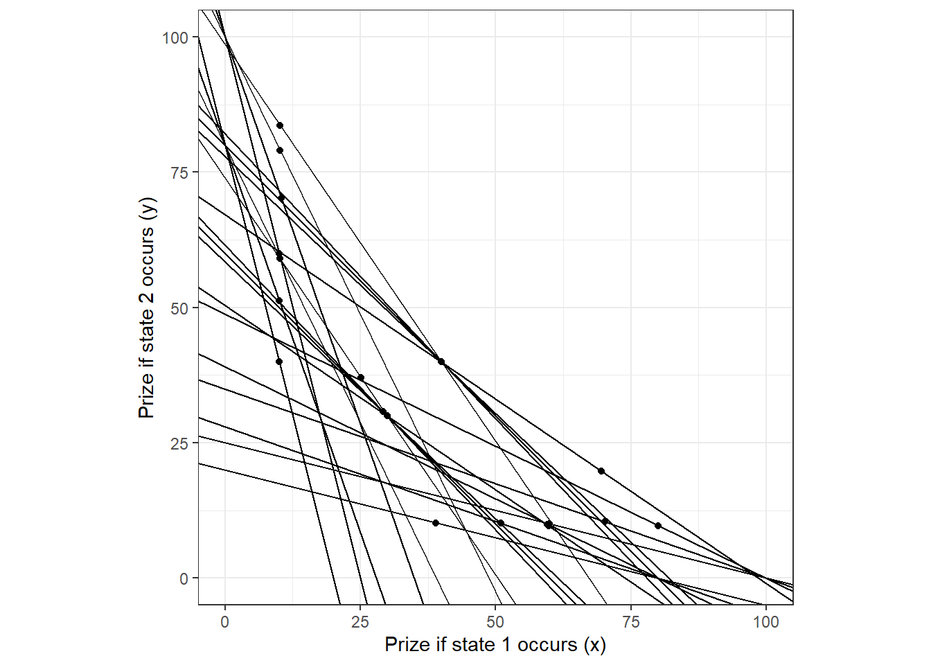
Budget sets and choices of one participant in @Halevy2018

Figure 3.1: Budget sets and choices of one participant in Halevy, Persitz, and Zrill (2018)

Each budget set is characterized in th data by the $y$- and $x$-intercepts of the budget line, so if we denote these as $\bar y_t$ and $\bar x_t$ respectively for budget set $t$, then we can write the budget as:

\[ \begin{aligned} y&=\bar y_t-x\frac{\bar y_t}{\bar x_t} \end{aligned} \]

Let’s suppose each participant is an expected utility maximizer with a constant relative risk aversion utility function over certain amounts of money:

\[ u_i(x)=\frac{x^{1-r}}{1-r} \]

Then the participant’s utility maximization problem is:

\[ \begin{aligned} \max_{x,y\geq 0}\left\{0.5\frac{x^{1-r}}{1-r}+0.5\frac{y^{1-r}}{1-r}\right\}\quad \text{s.t.: } y=\bar y_t-x\frac{\bar y_t}{\bar x_t} \end{aligned} \]

We can set up a Lagrangian to solve for the optimal portfolio choice (again, forgive me, I like to show my working):

\[ \begin{aligned} \mathcal L&=0.5\frac{x^{1-r}}{1-r}+0.5\frac{y^{1-r}}{1-r} - \gamma\left(y_t-x\frac{\bar y_t}{\bar x_t}-y\right)\\ ~\\ 0&=0.5x^{-r}+\gamma\frac{\bar y_t}{\bar x_t}\\ 0&=0.5 y^{-r}+\gamma\\ ~\\ -2\gamma&=x^{-r}\frac{\bar x_t}{\bar y_t}=y^{-r}\\ \left(\frac yx\right)^{-r}&=\frac{\bar x_t}{\bar y_t}\\ \frac{y}{x}&=\left(\frac{\bar y_t}{\bar x_t}\right)^{\frac{1}{r}} \end{aligned} \]

Substituting this into the budget constraint yields:

\[ \begin{aligned} x\left(\frac{\bar y_t}{\bar x_t}\right)^{\frac{1}{r}}&=\bar y_t-x\frac{\bar y_t}{\bar x_t}\\ x\left(\left(\frac{\bar y_t}{\bar x_t}\right)^{\frac{1}{r}}+\frac{\bar y_t}{\bar x_t}\right)&=\bar y_t\\ x&=\frac{\bar y_t}{\left(\frac{\bar y_t}{\bar x_t}\right)^{\frac{1}{r}}+\frac{\bar y_t}{\bar x_t}}\\ y&=\frac{\bar y_t\left(\frac{\bar y_t}{\bar x_t}\right)^{\frac{1}{r}}}{\left(\frac{\bar y_t}{\bar x_t}\right)^{\frac{1}{r}}+\frac{\bar y_t}{\bar x_t}} \end{aligned} \]

So our deterministic model of behavior is:

\[ \begin{aligned} x^*(\bar x_t,\bar y_t)&=\frac{\bar y_t}{\left(\frac{\bar y_t}{\bar x_t}\right)^{\frac{1}{r}}+\frac{\bar y_t}{\bar x_t}}\\ y^*(\bar x_t,\bar y_t)&=\frac{\bar y_t\left(\frac{\bar y_t}{\bar x_t}\right)^{\frac{1}{r}}}{\left(\frac{\bar y_t}{\bar x_t}\right)^{\frac{1}{r}}+\frac{\bar y_t}{\bar x_t}} \end{aligned} \]

3.4 Optimal choice plus an error

One common approach to turning a deterministic model into a probabilistic model, especially in these convex budget set experiments, is to add a mean-zero error term to these deterministic predictions. That is, on average the participant chooses $(x^*,y^*)$, but then each decision is implemented with an error. A simple specification for this is to assume that the error term is normally distributed:

\[ x\mid x^*\sim N(x^*,\sigma^2) \]

If we were using Frequentist techniques, this is where we might go ahead and estimate the model using nonlinear least squares, as is done in Andreoni and Vesterlund (2001), Andreoni and Miller (2002), and for one of the estimators under consideration in Halevy, Persitz, and Zrill (2018). For the Bayesian application, and for the maximum likelihood application for that matter, we need to be careful about a few things here.⁵

Firstly, the choice of whether to use $x$ or $y$ as our dependent variable is not inconsequential. To see this, note that since most of the lines in Figure 3.1 do not have a slope of negative one, the probabilistic predictions will be different between these two specifications. That is, if we choose $x$ as our explanatory variable, then it must be that:

\[ y\mid y^*\sim N\left(y^*,\left(\frac{\bar y_t}{\bar x_t}\right)^2\sigma^2\right) \]

So the variance of $y$ is not the same as the variance of $x$. Perhaps more alarmingly, the variance of $y$ is a function of the slope of the budget set, but the variance of $x$ is constant, so choices of $y$ will be more or less precise as these budget lines shift. Thus, homoskedasticity in x implies heteroskedastcity in y. This specification therefore suffers from a labeling problem, and we will likely end up with different estimates depending on whether we choose $x$ or $y$ as our explanatory variable.

Another modeling issue to consider is whether the distribution $x\mid x^*$ is truncated or censored at the endpoints of the choice set. For example, what happens to our prediction if $x^*=3$ but our error term implies that $x=-5$? Such a realization is possible with a normal distribution, but it is a choice that the experiment would have prevented the participant from choosing. For example, let’s simulate some draws assuming $x\sim N(1,2)$, and consider the implications of getting some draws with $x<0$, which the experiment would not allow a participant to choose:

dx <- tibble(x=rnorm(10000,mean=1,sd=sqrt(2)))
dsim<-rbind(
  dx %>% mutate(type = "Normal"),
  dx %>% filter(x>=0) %>% mutate(type="truncated"),
  dx %>% mutate(x=ifelse(x<0,0,x)) %>% mutate(type="censored")
)
(
  ggplot(dsim,aes(x=x))
  +geom_histogram()
  +facet_wrap(~type)
  +theme_bw()
)

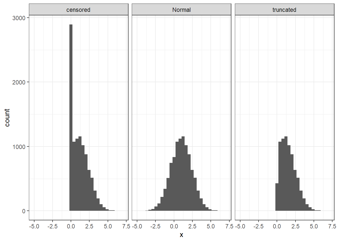
Figure 3.2: Examples of censored and truncated data.

Figure 3.2 illustrates the difference between censoring and truncation. Firstly, the un-censored, un-truncated simulated data is shown in the middle panel. Clearly these could not be choices from a convex budget set problem, because the participant would sometimes choose a negative amount of $x$. The left panel shows what happens when the data are censored at zero. All observations with $x<0$ are coded as $x=0$, and we can see that this is happening because there is a spike in the distribution at $x=0$. Truncation, on the other hand, is shown in the rightmost panel. Here we see no spike because instead of coding all negative numbers as zeros, they are simply thrown out. The choice of which specification to go with here should be specific to the application. For example, in experiments investigating other-regarding preferences such as Andreoni and Vesterlund (2001) and Andreoni and Miller (2002), it is likely that there will be a substantial fraction of selfish participants who pass no money to their partner. In this case a spike of data at zero makes a lot of sense. For the Halevy, Persitz, and Zrill (2018) experiment, on this other hand, choosing $x=0$ means that the participant wants to earn nothing in one of the two, equally likely, states of the world. This seemed unlikely to me, but we can look at the data to see how uncommon this is:

tab<-(D
  |> group_by(`X-intercept`,`Y-intercept`)
  |> summarize(`fraction choosing zero` = mean(X==0 | Y==0))
  
)
tab|> knitr::kable(caption="Fraction of participants choosing either $x=0$ or $y=0$ in each of the 22 budget sets in @Halevy2018.")

Table 3.1: Fraction of participants choosing either $x=0$ or $y=0$ in each of the 22 budget sets in Halevy, Persitz, and Zrill (2018).
X-intercept	Y-intercept	fraction choosing zero
20.00	80.00	0.2898551
25.00	100.00	0.3285024
27.94	80.00	0.2463768
34.92	100.00	0.3043478
39.03	80.00	0.1739130
48.79	100.00	0.2222222
50.45	74.00	0.0821256
58.50	61.57	0.0144928
60.00	60.00	0.0193237
61.57	58.50	0.0193237
67.26	98.67	0.1159420
74.00	50.45	0.0869565
78.00	82.10	0.0193237
80.00	20.00	0.2995169
80.00	27.94	0.2318841
80.00	39.03	0.1739130
80.00	80.00	0.0144928
82.10	78.00	0.0241546
98.67	67.26	0.1062802
100.00	25.00	0.2946860
100.00	34.92	0.2415459
100.00	48.79	0.1932367

Table 3.1 proves me wrong! There are in fact a substantial minority of participants in some budgets sets who choose zero. I will take this onboard with the modeling presented below.⁶ In particular, I will implement the censoring specification, rather than the truncation specification.

3.4.1 Estimating a model

For the purposes of this example, I will make some simplifying assumptions. These are mainly to speed up computation. Halevy, Persitz, and Zrill (2018) allow their participants to choose in increments of 0.2 tokens, so if I was being truly faithful to the data-generating process, I would be modeling the choice set as a grid with resolution 0.2. In the interest of making the task less strenuous for my laptop, I normalize the budget sets by dividing by the $x$ intercept, so the choice of $x$ must be on the unit interval. I then round the normalized $x$ choices to the nearest 0.05 units.⁷ The information I will pass to Stan will be the normalized $y$-intercept, and the range that the normalized choice fell into:

gridsize<-0.05

d<-(
  d
  |> mutate(x= X/`X-intercept`,
            yint = `Y-intercept`/`X-intercept`,
            xgrid = floor(x/gridsize),
            # lower and upper bounds for the censored data
            xlb = xgrid*gridsize,
            xub = (xgrid+1)*gridsize,
            
            # This ensures that the lower and upper bounds at the endpoints of
            # the grid are (-999,0.05) and (0.95,999)
            xlb = ifelse(x==0,-999,xlb),
            xlb = ifelse(x==1,1-gridsize,xlb),
            xub = ifelse(x==1,999,xub)
            )
  
)

That is, if a participant chose, say, a (normalized) $x=0.23$, I will use the information that $0.20<x<0.25$. That is, xlb=0.20 and xub=0.25 The probability of a choice $x$ being in this region $(x_{lb},x_{ub})$ is then:

\[ \Pr\left(x_{lb}<x<x_{ub}\right)=\Phi\left(\frac{x_{ub}-x^*}{\sigma}\right)-\Phi\left(\frac{x_{lb}-x^*}{\sigma}\right) \]

where $\Phi(\cdot)$ is the standard normal cumulative density function. For decisions that were at the endpoints of the choice set, I set $x_{lb}=-999$ if $x=0$, and $x_{ub}=999$ if $x=1$.

Here is the Stan file I use:


data {
  int<lower=0> n; // number of observations
  real xlb[n]; // lower bound for x choice
  real xub[n]; // upper bound for x choice
  real yint[n]; // y intercept
  
  real prior_r[2];
  real prior_sigma;
}


parameters {
  real r;
  real<lower=0> sigma;
}

model {
  
  real xstar[n];
  real px[n];
  
  for (ii in 1:n) {
    // optimal choice given r
    xstar[ii] = yint[ii]/ (pow(yint[ii],1.0/r)+yint[ii]);
    // probability of the optimal choice + error landing where it did
    px[ii] = normal_cdf(xub[ii],xstar[ii],sigma)-normal_cdf(xlb[ii],xstar[ii],sigma);
  }
  
  
  // increment the likelihood
  target +=log(px);
  
  // priors
  r ~ normal(prior_r[1],prior_r[2]);
  sigma ~ cauchy(0.0,prior_sigma);
  
  
}

Here’s how we estimate it for the one participant:

library(rstan)
rstan_options(auto_write = TRUE)
options(mc.cores = parallel::detectCores())

dStan<-list(
  n = dim(d)[1],
  xlb = d$xlb,
  xub = d$xub,
  yint = d$yint,
  
  prior_r = c(0.5,0.25),
  prior_sigma = 0.008
)

if (!file.exists("Outputs/ProbabilisticModels/ProbMods_HPZ2018_normal.rds")) {
  Fit<-stan("Code/ProbabilisticModels/ProbMods_HPZ2018_normal.stan",
            data=dStan,seed=42)
  # Save the fitted model results
  saveRDS(Fit,file = "Outputs/ProbabilisticModels/ProbMods_HPZ2018_normal.rds")
}
# load the fitted model results
FitNormal<-readRDS("Outputs/ProbabilisticModels/ProbMods_HPZ2018_normal.rds")


summary(FitNormal)$summary |> knitr::kable(caption="Posterior estimates  of the 'optimal choice plus error' model.")

Table 3.2: Posterior estimates of the ‘optimal choice plus error’ model.
	mean	se_mean	sd	2.5%	25%	50%	75%	97.5%	n_eff	Rhat
r	0.6356843	0.0016724	0.0740045	0.5014449	0.5854661	0.6313009	0.6819358	0.7911945	1958.047	1.001512
sigma	0.1429142	0.0004520	0.0226142	0.1066118	0.1265328	0.1403869	0.1564103	0.1948155	2503.575	0.999256
lp__	-62.5379703	0.0278744	1.0820914	-65.2606211	-62.9812424	-62.2161067	-61.7512873	-61.4540023	1507.011	1.001079

The estimates in Table 3.2 seem plausible based on what we know about participants in economic experiments. $r\approx 0.63$ is right in the meaty part of the distribution of typical levels of risk aversion for experiment participants, and $\sigma\approx 0.14$ means that choices are not so noisy that they always get censored at zero or one.

3.5 Utility-based models

Another approach for going from a deterministic to a probabilistic model is to have the utility function determine the entire probability distribution of our data. Note that for the “optimal choice plus error” model, the only place that the utility function came into the equation was in determining where the distribution of choices was centered. To show you why this might be a problem, let’s look a bit deeper into what the participant’s utility maximization problem looks like for one decision in Halevy, Persitz, and Zrill (2018). In particular, here is what their utility of choosing an allocation $\left(x,(1-x)\bar y/\bar x\right)$ looks like for the normalized budget set when $\bar y/\bar x = 4$:

ybar<-4
r<-0.5
d<-(
  tibble(x=seq(0.001,0.999,length=101))
  |> mutate(utility = 0.5*x^(1-r)/(1-r)+0.5*((1-x)*ybar)^(1-r)/(1-r)
            )
)
optimal<-d$x[which.max(d$utility)]
(
  ggplot(d)
  +geom_path(aes(x=x,y=utility))
  +geom_vline(xintercept=optimal,color="red")
  +theme_bw()
  +ylab("Expected utility")
)

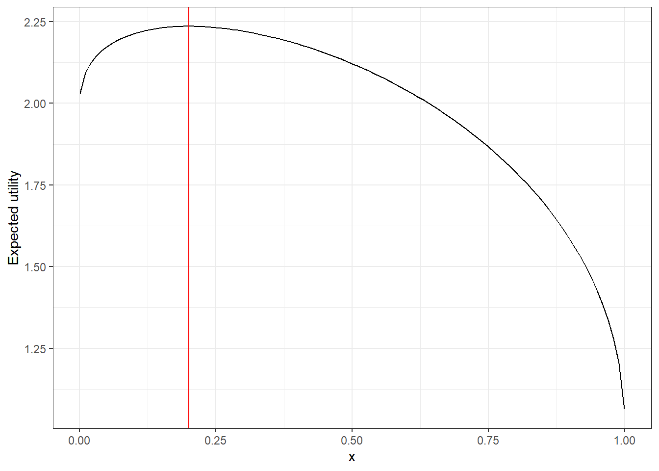
$The expected utility function in @Halevy2018 for a participant with $r=0.5$ when $\bar y/\bar x=4$. The vertical red line denotes the optimal choice$

Figure 3.3: The expected utility function in Halevy, Persitz, and Zrill (2018) for a participant with $r=0.5$ when $\bar y/\bar x=4$. The vertical red line denotes the optimal choice

One important feature of Figure 3.3 is that the expected utility function is not symmetric: there is a much sharper drop-off in utility moving to the left of the optimal choice (red line) than to the right. Yet the “optimal choice plus error” model will assume a symmetric distribution centered on the red line (outside of any censoring or truncation). This is because that model does not take into account the shape of this plot, only the maximum.

This goes against a lot of our understanding of how actual humans make decisions. In particular, they are more likely to take actions that yield higher utility than those that yield lower utility. In order for our model to reflect this, then loosely speaking, what we want for our probabilistic model to look something like this:

\[ p\left(y\mid x, \theta\right)=g\left(U(y,x;\theta)\right) \]

with $g'(u)>0$. That is, the probability of choosing an action is increasing in the utility associated with taking that action.

By far the most common implementation of this is the logistic choice rule, which mathematically looks like this:

\[ p(y\mid x,\theta)=\frac{\exp\left(\lambda U(y,x;\theta)\right)}{\sum_{z\in\mathbb Y}\exp\left(\lambda U(z,x;\theta)\right)} \] where $\lambda>0$ measures a participant’s choice precision: as $\lambda$ increases, the participant is more sensitive to payoffs. For this decision in Halevy, Persitz, and Zrill (2018), the probabilistic predictions from logit choice look like this:⁸

LAMBDA<-c(1,10,30,40)
dlogit<-tibble()

for (ll in LAMBDA) {
  tmp<-(d
    |> mutate(
              lu = ll*utility,
              px = exp(lu-max(lu))/sum(exp(lu-max(lu))),
              lambda = paste("\u03bb =",ll)
              )  
  )
  dlogit<-rbind(dlogit,tmp)
}

(
  ggplot(dlogit,aes(x=x,y=px,linetype=lambda))
  +geom_path()
  +geom_vline(xintercept=optimal,color="red")
  +ylab("probability")
  +theme_bw()
)

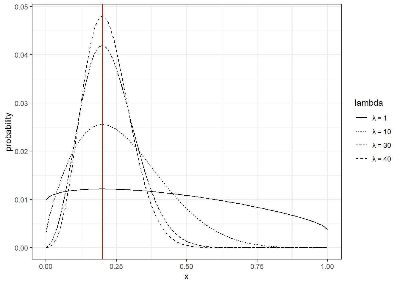
$Logistic choice in @Halevy2018 for a participant with $r=0.5$ when $\bar y/\bar x=4$. The vertical red line denotes the optimal choice$

Figure 3.4: Logistic choice in Halevy, Persitz, and Zrill (2018) for a participant with $r=0.5$ when $\bar y/\bar x=4$. The vertical red line denotes the optimal choice

In particular, the distributions in Figure 3.4 are not symmetric: they have a longer right tail than left tail. This is because making “mistakes” by choosing slightly to the right of the optimal choice (red line) are less costly than choosing slightly to the left.

3.5.1 Estimating a model

Here is the Stan file for estimating this logistic choice model. As with the previous model, I need to discretize the choice set. For this implementation, instead of just computing a point prediction and adding an error, I need to compute utility for every possible choice that could be made. This is done over the grid veriable xgrid, and the element of this grid that most closely matches the participant’s choice is xi.


data {
  int<lower=0> n; // number of observations
  int gridsize;
  vector[gridsize] xgrid; // grid to discretize choice of x over
  int xi[n]; // index for the grid for choice of x
  
  real yint[n]; // y intercept
  
  real prior_r[2];
  real prior_lambda;
}


parameters {
  real r;
  real<lower=0> lambda;
}

model {
  

  
  for (ii in 1:n) {
    vector[gridsize] EU;
    vector[gridsize] probX;
    
    // expected utility of choosing each x in the grid
    EU = 0.5*pow(xgrid,1.0-r)/(1.0-r)+0.5*pow((1.0-xgrid)*yint[ii],1.0-r)/(1.0-r);
    
    // logit choice probabilities
    probX = log_softmax(lambda*EU);
    
    // increment the likelihood by the log probability chosen
    target += probX[xi[ii]];
    
  }
  
  // priors
  r ~ normal(prior_r[1],prior_r[2]);
  lambda ~ cauchy(0.0,prior_lambda);
  
  
}

And here is how I pass the data to Stan to estimate the model in R:

gridsize<-20
Xgrid <- seq(1/(2*gridsize),1-1/(2*gridsize),by=1/gridsize)
d<-(
  d
  %>% rowwise()
  %>% mutate(xi = which.min(abs(x-Xgrid)))
)

dStan<-list(
  n = dim(d)[1],
  xgrid = Xgrid,
  gridsize=gridsize,
  xi=d$xi,
  yint = d$yint,
  
  prior_r = c(0.5,0.25),
  prior_lambda = 0.08
)

## Warning: Unknown or uninitialised column: `yint`.

if (!file.exists("Outputs/ProbabilisticModels/ProbMods_HPZ2018_logit.rds")) {
  Fit<-stan("Code/ProbabilisticModels/ProbMods_HPZ2018_logit.stan",
            data=dStan,seed=42)
  # Save the fitted model results
  saveRDS(Fit,file = "Outputs/ProbabilisticModels/ProbMods_HPZ2018_logit.rds")
}
# load the fitted model results
FitLogit<-readRDS("Outputs/ProbabilisticModels/ProbMods_HPZ2018_logit.rds")


summary(FitLogit)$summary |> knitr::kable(caption="Posterior estimates of the logit choice model.")

Table 3.3: Posterior estimates of the logit choice model.
	mean	se_mean	sd	2.5%	25%	50%	75%	97.5%	n_eff	Rhat
r	0.6180463	0.0022409	0.0823109	0.479191	0.5672429	0.6121625	0.6612087	0.7932096	1349.1623	1.003993
lambda	19.4787417	0.2092722	8.1674884	5.569901	13.7510580	18.7127683	24.4728880	37.7761375	1523.1894	1.001866
lp__	-61.6231103	0.0584521	1.3736571	-65.357691	-62.0096403	-61.1958480	-60.7450303	-60.4548983	552.2771	1.006458

The posterior estimates are summarized in Table 3.3. While we cannot directly compare the parameters $\lambda$ and $\sigma$, we can compare the estimates of the risk-aversion parameter $r$. These are both similar in terms of the posterior mean and the posterior standard deviation.

3.5.2 Doing something with the estimates

While having and estimate of $r$ and $\lambda$ might be useful to your research question on their own, note that because they are parameters of a probabilistic choice model, they can be used to make predictions and derive implications. To fix ideas, let’s just focus on the first decision that this participant made. For this decision, the normalized $y$ intercept of the budget line was yint=0.3492, and they chose to invest a normalized amount of x=0.702 in the asset that pays out in State 1. Let’s begin by extracting our estimated model’s posterior draws, and then we will use them to derive some predictions.

postdraws<-tibble(r=extract(FitLogit)$r,lambda=extract(FitLogit)$lambda)

(
  ggplot(postdraws,aes(x=r,y=lambda))
  +geom_point(size=0.3)
  +theme_bw()
  +ylab("\u03bb")
)

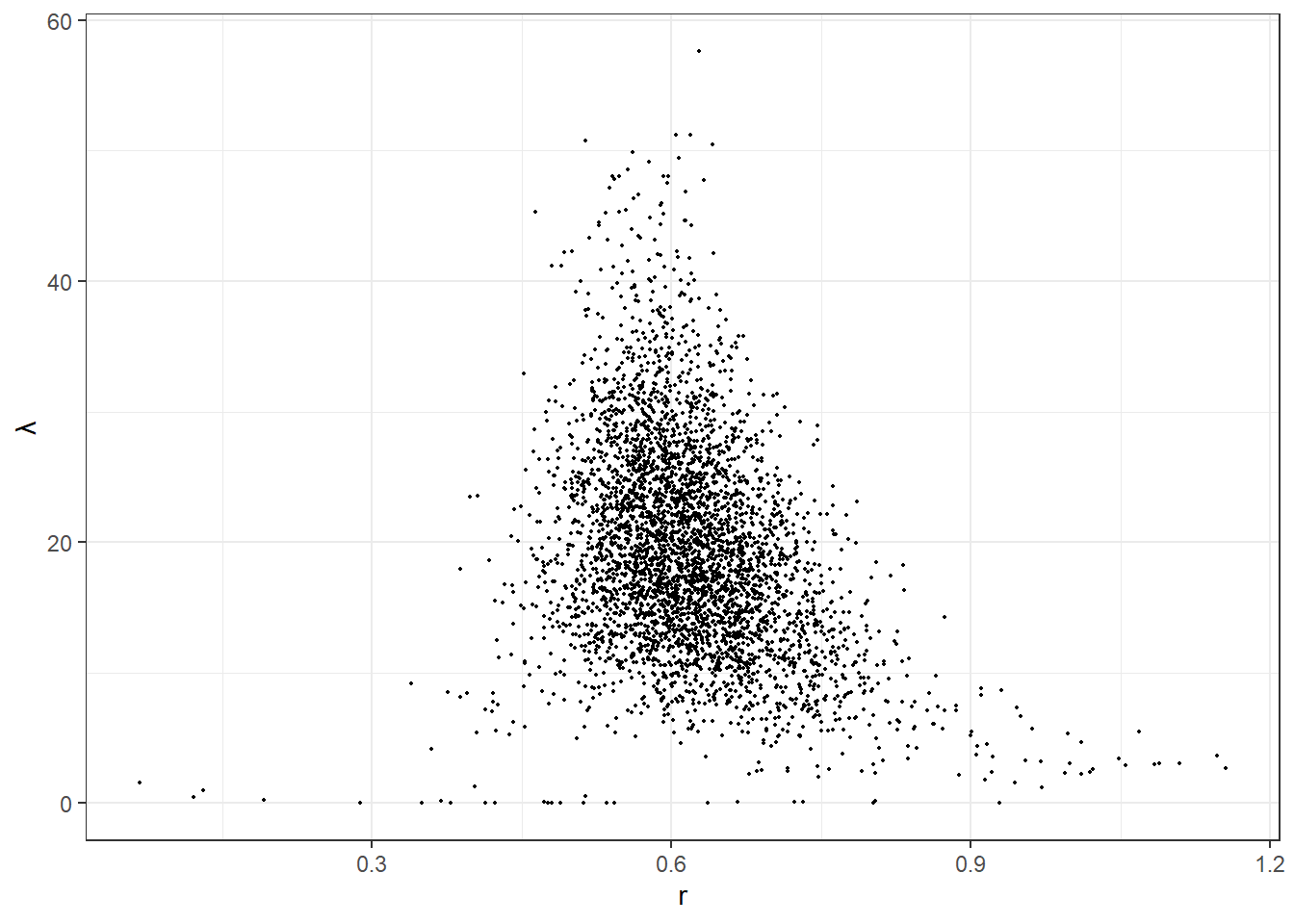
Figure 3.5: Posterior draws from the estimated logit choice model

Firstly, let’s look at our model’s prediction for this decision. Recall that since we estimated a probabilistic model, our models prediction will be a probability distribution. Furthermore, since we have 4,000 draws from the posterior distribution, we will have 4,000 posterior draws of this probability distribution. Here is what I came up with the visualize the model’s prediction for this choice

yint<-0.3492

ProbPrediction<-tibble()

for (ss in 1:dim(postdraws)[1]) {
  r<-postdraws[ss,]$r
  lambda<-postdraws[ss,]$lambda
  
  EU<-0.5*Xgrid^(1-r)/(1-r)+0.5*((1-Xgrid)*yint)^(1-r)/(1-r)
  Pr<-exp(lambda*EU-max(lambda*EU))/sum(exp(lambda*EU-max(lambda*EU)))
  ProbPrediction<-rbind(ProbPrediction,tibble(x=Xgrid,Pr=Pr))
}

means<-ProbPrediction |> group_by(x) |> summarize(meanPr = mean(Pr))

(
  ggplot()
  +geom_jitter(data=ProbPrediction,aes(x=x,y=Pr),size=0.2,alpha=0.1)
  +geom_line(data=means,aes(x=x,y=meanPr),color="red",linewidth=2)
  +theme_bw()
  +geom_vline(xintercept=0.702,color="blue",linewidth=2,linetype="dashed")
  +xlab("Investment in the state 1 asset")
  +ylab("Probability")
)

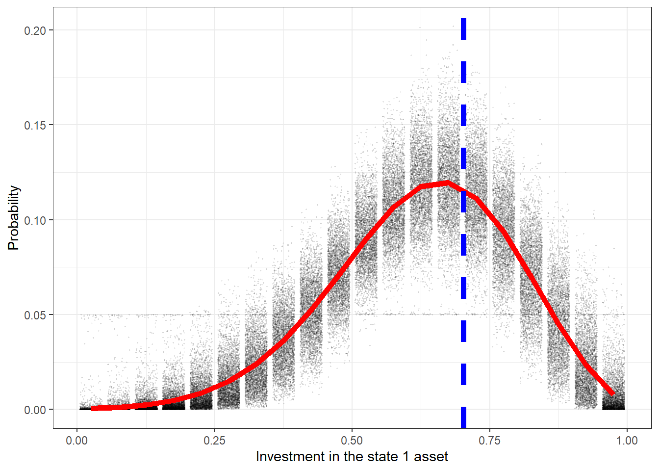
Posterior predictive distribution for the participant. Dots show draws from the individual posterior distribution. The red curve shows the mean of this predictive distribution. The dashed blue line shows the choice that was made by the participant.

Figure 3.6: Posterior predictive distribution for the participant. Dots show draws from the individual posterior distribution. The red curve shows the mean of this predictive distribution. The dashed blue line shows the choice that was made by the participant.

So it looks like the participant chose fairly closely (blue line) to what our model estimated was their optimal choice.⁹

Finally, whenever I see a plot like Figure 3.1, I always wonder what the indifference curves look like. So in the interest of satisfying my curiosity, let’s work out what their indifference curve looks like for the choice that they made. To begin with, the equation of the indifference curve is:

\[ \begin{aligned} \bar u&=0.5\frac{x^{1-r}}{1-r}+0.5\frac{y^{1-r}}{1-r}\\ y^{1-r}&=2(1-r)\bar u-x^{1-r}\\ y&=\left(2(1-r)\bar u-x^{1-r}\right)^{\frac{1}{1-r}} \end{aligned} \]

where $\bar u$ is the utility of the indifference curve. Let’s work out what the indifference curves look like using our 4,000 posterior draws:

indiff<-(
  expand.grid(r = postdraws$r,x=seq(0.1,0.9,length=20))
    |> mutate(
      ubar = 0.5*0.702^(1-r)/(1-r)+0.5*((1-0.702)*0.3492)^(1-r)/(1-r),
      y = (2*(1-r)*ubar-x^(1-r))^(1/(1-r))
    )
  |> group_by(x)
  |> summarize(mean=mean(y),
               p05=quantile(y,probs=0.05,na.rm=T),
               p95=quantile(y,probs=0.95,na.rm=T),
               p25=quantile(y,probs=0.25,na.rm=T),
               p75=quantile(y,probs=0.75,na.rm=T)
               )
)

(
  ggplot(indiff,aes(x=x))
  +geom_abline(slope = -0.3492,intercept = 0.3492,linewidth=1)
  +geom_ribbon(aes(ymax=p95,ymin=p05),alpha=0.2)
  +geom_ribbon(aes(ymax=p75,ymin=p25),alpha=0.4)
  +geom_line(aes(y=mean))
  +theme_bw()
  +xlab("Prize if state 1 occurs (x)")+ylab("Prize if state 2 occurs (y)")
  +geom_text(x=0.702,y=0.349*(1-0.702),label="X")
)

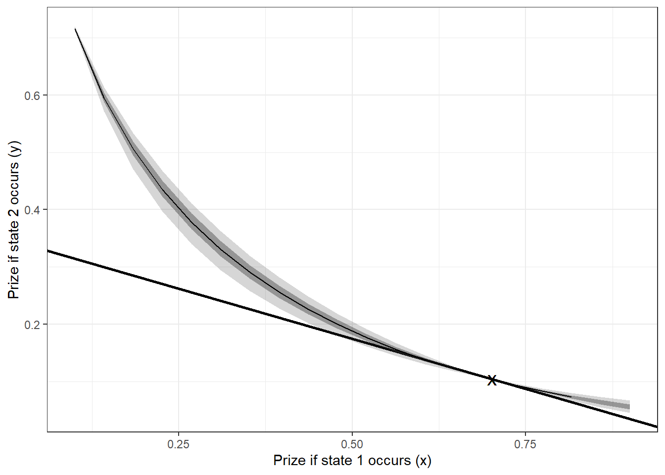
Estimated indifference curve of the first choice made by the participant. Shaded areas show 50% and 95% Bayesian credible regions. X denotes the choice made by the participant.

Figure 3.7: Estimated indifference curve of the first choice made by the participant. Shaded areas show 50% and 95% Bayesian credible regions. X denotes the choice made by the participant.

Figure 3.7 shows the estimated indifference curve for this first decision, Including 95% and 50% Bayesian credible regions around its point prediction. Note that in this process, once we have draws from the posterior, it is very easy not just to get point predictions that are transforms of our parameters (like this indifference curve), but also the entire posterior distribution of these transforms. This will be extremely useful to us, as our structural models’ predictions are often nonlinear transformations of the parameters. Other quantities as well, such as utility, indifference curves, reservation values, and so on, are just as easily computed.

References

Andreoni, James, and John Miller. 2002. “Giving According to GARP: An Experimental Test of the Consistency of Preferences for Altruism.” Econometrica 70 (2): 737–53. https://www.jstor.org/stable/2692289.

Andreoni, James, and Lise Vesterlund. 2001. “Which Is the Fair Sex? Gender Differences in Altruism.” The Quarterly Journal of Economics 116 (1): 293–312. https://doi.org/10.1162/003355301556419.

Halevy, Yoram, Dotan Persitz, and Lanny Zrill. 2018. “Parametric Recoverability of Preferences.” Journal of Political Economy 126 (4): 1558–93. https://doi.org/10.1086/697741.

Here I say “likelihood-based”, because the argument applies to any technique that uses a likelihood. Bayesian estimation and Maximum likelihood estimation both use a likelihood.↩︎
There are a few reasons for this. For one thing, for pedagogical reasons I want to keep the examples in this chapter as simple as possible. Going to more than one participant will complicate matters both computationally and conceptually. We will cover these issues later. Also, Stan returns some errors when I estimate these models for many of the other participants, and instead of giving attention to how to understand and address these errors here, I prefer to show you what you can do with a probabilistic model. We will get to understanding and fixing Stan’s error warnings later.↩︎
I am not saying that nonlinear least squares avoids these problems, just that the problems become more apparent when one is dealing directly with a likelihood.↩︎
I acknowledge that I am being a bad Bayesian in that I have looked at the data before estimating my model here. It probably would have been better to estimate both models (truncation and censoring), and then assess which one is matching the data better.↩︎
This is another kind of censoring: I know that the actual choice falls within a range, but I do not know where in the range the actual choice was.↩︎
Note that when I computed the logit choice probabilities in Figure 3.4, I first subtracted the maximum utility. This does not mathematically change the answer, but computationally is much more stable because we avoid exponentiating large positive numbers.↩︎
We should be wary of using this as evidence that we have a good fit for our model, because this participant’s choice was used in estimating the model. In a later chapter I will discuss some cross-validation techniques that can be used to assess goodness of fit.↩︎