6 Hierarchical models
6.1 A random sample of participants walks into your lab
Suppose that your goal was to estimate a parameter \(\theta_i\) for every participant in your experiment. In an ideal world, they would come into your laboratory with \(\theta_i\) stamped to their face, and all you would have to do to know it perfectly would be to briefly look at them, pay them a small show-up fee, take note of their \(\theta_i\), and send them on their way. Such ideal participants are a pipe dream, but what we can do is ask them to make decisions \(y_i\) that reveal to us something about their \(\theta_i\). If we have a probabilistic model that relates \(y_i\) to \(\theta_i\), and we have a prior for \(\theta_i\), then we can learn about \(\theta_i\). But \(i\) is not the only participant who comes to the lab. \(j\), \(k\), and \(l\) do as well. In fact, we are fortunate enough to get \(n\) of them! Is there anything we can learn about \(\theta_i\) by studying the data from participants \(j\), \(k\), and \(l\)? The answer to this is a definitive “yes”, if \(\theta_i\), \(\theta_j\), \(\theta_k\), and \(\theta_l\) are all drawn from the same distribution. In economic experiments this is a reasonably good assumption, as participants are typically drawn from the same subject pool.
So how do we learn about \(\theta_i\) from \(j\)’s decisions? We note that \(\theta_i\) and \(\theta_j\) are both draws from the same distribution, and so decisions \(y_j\) are informative of not just \(\theta_j\), but the parameters governing this population-level distribution, call them \(\mathcal P\). That is, knowing \(\mathcal P\) helps us learn about \(\theta_j\) because \(\mathcal P\) is the prior we should have on \(\theta_i\), and \(y_j\) tells us something about \(\theta_j\), which in turn tells us something about \(\mathcal P\). So even if we don’t care directly about \(\mathcal P\), \(j\)’s decisions can help us learn about \(i\)’s parameter, if we let them. Furthermore, learning about population-level parameters \(\mathcal P\) might be more interesting to us as researches than whatever is going on at the individual level. These parameters allow us to extrapolate beyond the sample of participants we get, and make statements about our entire subject pool.
This is where the benefits of Bayesian estimation really start to be realized!
Up to this point we have focused solely on representative agent models and participant-specific models. All of this work has not been a waste, as these models are important stepping stones on the way to richer models, but it is these richer models that provide deeper insight into our data. In this chapter, we will be estimating population-level parameters. These are parameters that govern the distribution of (what are usually) our participants’ individual parameters. That is, if our economic model is about preferences, we will be estimating the distribution of preferences. This is an amazingly powerful tool.
We will do this by assuming that our data follows a hierarchical structure. By that I mean that we will assume that we can partition our data into chunks, and maybe even that we can further partition these chunks into sub-chunks. We will then add some structure to how these chunks are related to each other, and estimate these relationships. What we get out of this is a quantification of the heterogeneity that exists between these chunks, and if we have more than one level (i.e. chunks and sub-chunks), the relative contribution to heterogeneity of each level.
6.2 The anatomy of a basic hierarchical model
In the previous chapter, we estimated a participant’s parameters using just the data generated by that participant. Specifically, we focused on just their own data \(y_i\), while ignoring the data produced by all our other participants \(y_{-i}\). Just like these participant-specific models, we will continue to have a probabilistic model for the participant’s behavior, which we will denote as the likelihood \(p(y_i\mid\theta_i)\). However now we will further specify a distribution for \(\theta_i\). That is, we will assume that each participant’s \(\theta_i\) is an independent draw from the population of potential participants:
\[ \theta_i\sim iid G(\mathcal P) \]
where \(G\) is the family of distribution we have chosen to model how the \(\theta_i\)s are generated, and \(\mathcal P\) are the parameters in the distribution \(G\). For example, probably the most popular hierarchical specification assumes that \(\theta_i\) are drawn from a multivariate normal distribution, so \(\mathcal P=(\mu,\Sigma)\) are the mean vector and variance-covariance matrix of this distribution. I will discuss the multivariate normal hierarchical model in much more detail below.
If we were lucky enough to just observe \(\theta_i\), then it would be a straightforward task estimating \(\mathcal P\). Instead though, we get data that are generated according to:
\[ y_i\sim g(\theta_i) \] where \(g\) is the family of distribution that we have chosen to model how our data \(y_i\) are generated conditional on our participant’s parameter \(\theta_i\). Putting this together, we observe \(y_i\), which tells us something about \(\theta_i\), which tells us something about \(\mathcal P\).
Note that all we need to simulate this data-generating process is to specify \(\mathcal P\). That is, we can:
- Draw \(\theta_i\sim G(\mathcal P)\), then
- Draw \(y_i\sim g(\theta_i)\)
Therefore, our likelihood for a participant’s data can be defined as follows:
\[ \begin{aligned} p(y_i,\theta_i\mid \mathcal P)&=p(y_i\mid \theta_i,\mathcal P)p(\theta_i\mid \mathcal P)\\ &=p(y_i\mid\theta_i)p(\theta_i\mid\mathcal P) \end{aligned} \]
where the second line follows if we assume that \(y_i\) and \(\mathcal P\) are independent conditional on \(\theta_i\). In plainer English: once we know \(\theta_i\), \(\mathcal P\) will tell us no more information about \(y_i\). The power of this assumption is that it allows us to think separately about how our data are generated given the participant’s parameters, (i.e. \(p(y_i\mid\theta_i)\)), and how participants are distributed across the population (i.e. \(p(\theta_i\mid\mathcal P)\)).
Conceptually, the hierarchical structure (a distribution for \(\theta_i\)) is hopefully easy to grasp. However we have a practical problem: we still don’t know \(\theta_i\), so any expression that includes it cannot be feasibly used to evaluate our model’s likelihood. The next section will develop two techniques for doing this. The first, integrating the likelihood, is popular for Frequentist techniques, but may sometimes be useful in Bayesian applications too; and the second, data augmentation, is the typical Bayesian go-to for this problem, and lends itself especially to the Hamiltonian Monte Carlo of Stan (Betancourt and Girolami 2015).
6.3 Accounting for unobserved heterogeneity
One of the hurdles I came accross when I started learning about hierarchical models was how to treat unobservable heterogeneity. For most of the models discussed in this book, this unobservable heterogeneity will mostly be in participant-specific parameters. This problem is not specific to Bayesian implementations of hierarchical models, but it is typically addressed differently depending on whether one adopts a Bayesian or Frequentist (maximum likelihood) approach. In both cases the models can make the same distributional assumptions about \(\theta\), but they are typically treated in very different ways.
While maximum likelihood techniques typically integrate out the unobserved heterogeneity \(\theta\) and just focus on estimating the population-level parameters \(\mathcal P\), the Bayesian implementation typically jointly estimates \(\theta\) alongside \(\mathcal P\). I include an introduction to both techniques, as I believe they can both be useful tools that might be the best option to you in some cases.
6.3.1 The last time you will integrate the likelihood, probably
The typical maximum likelihood implementation of a hierarchical model uses maximum simulated likelihood to eliminate the participant-level parameters \(\theta\) from the likelihood function. This technique in the context of economic experiments is discussed in Chapter 10 of Moffatt (2015), and is the implementation used in the hierarchical models estimated in, for example, Conte, Hey, and Moffatt (2011).
The likelihood of observing data \(y_i\) conditional on only population-level parameters \(\mathcal P\) can be approximated as:
\[ \begin{aligned} p(y_i\mid \mathcal P)&=\int_\Theta p(y_i,\theta\mid \mathcal P)\mathrm d\theta\\ &=\int_\Theta p(y_i\mid \theta,\mathcal P)p(\theta\mid\mathcal P)\mathrm d\theta\\ &=E_{\theta\mid\mathcal P}\left[p(y_i\mid\theta,\mathcal P)\right]\\ &\approx\frac{1}{S}\sum_{s=1}^S p(y_i\mid \theta^s,\mathcal P),\quad \text{with:}\ \theta^s\sim iid G(\mathcal P) \end{aligned} \]
where the first equality follows because of the relationship between the marginal distribution \(y_i\mid \mathcal P\) and the joint distribution \(y_i,\theta\mid \mathcal P\). The second inequality writes this joint distribution function as the product of a conditional and a marginal distribution.22 The third equality follows by recognizing that the expression in the second line is the expectation of \(p(y_i\mid \theta,\mathcal P)\), where \(\theta\mid\mathcal P\) is the only random variable, and the approximation is a Monte Carlo integration of this expectation. This approximation can be made more efficient using Halton draws, which are discussed in Section 10.3 of Moffatt (2015).
What all of this means is that you can approximate the likelihood of the entire dataset as:
\[ p(y\mid\mathcal P)=\prod_{i=1}^np(y_i\mid\mathcal P) \approx \prod_{i=1}^n\left(\frac{1}{S}\sum_{s=1}^Sp(y_i\mid \theta^s,\mathcal P)\right) \] So the log-likelihood function, which is what we would pass to Stan, is approximated as:
\[ \log p(y\mid \mathcal P)\approx\sum_{i=1}^n\log\left(\frac1S\sum_{s=1}^Sp(y_i\mid \theta^s,\mathcal P)\right) \]
6.3.2 Data augmentation
The other technique for accounting for unobserved heterogeneity is called “data augmentation”, and basically comes down to jointly estimating the participant-specific parameters alongside the population-level parameters. This means specifying a posterior distribution in the following form:
\[ \begin{aligned} p(\theta,\mathcal P\mid y)&\propto p(y\mid \theta,\mathcal P)p(\theta,\mathcal P)\\ &=p(y\mid \theta,\mathcal P)p(\theta\mid\mathcal P)p(\mathcal P) \end{aligned} \]
Note here the trade-off: we do not have to use Monte Carlo integration to approximate the likelihood (because we are jointly estimating \(\theta\)), but we now have a whole lot more parameters to estimate! Specifically, while we do not have to evaluate each likelihood \(S\) times for the Monte Carlo integration, we have to estimate all of the parameters in \(\theta\), not just \(\mathcal P\). As there will usually be at least one element in \(\theta\) for every participant, this means that data augmentation can have us going from a few to many parameters very quickly.
Our final product is the posterior draws of \(\mathcal P\) and \(\theta\), so not only do we have estimates of the population quantities, we also have estimates of the participants’ parameters. These estimates are referred to as shrinkage estimates because compared to their participant-specific counterparts from the previous section, they will be “shrunk” or pulled towards the center of the population distribution implied by \(\mathcal P\). This is a feature, not a bug: by jointly estimating \(\mathcal P\) alongside \(\theta\), we are allowing our data to decide for us what an appropriate prior for \(\theta\) is. In particular, this prior is the distribution implied by \(\mathcal P\), which since it is informed by the data, will most likely be more informative than our prior for the participant-specific counterpart.
The computational benefit of this method is that we only have to evaluate the likelihood once, instead of \(S\) times if we were integrating it. My intuition for this, albeit only informed through a lot of trial and error trying both methods with both maximum likelihood and Bayesian techniques, is that these methods are common in their respective statistical philosophies for computational practicalities. Hamiltonian Monte Carlo, which is what Stan does, seems to scale well with the number of parameters in the model. Hence, adding a whole lot of participant-specific \(\theta\)s to the bill of parameters that we need to estimate is not that much of an additional computational burden, especially when the \(\theta\)s are well informed by the “prior” in the population distribution \(\mathcal P\). On the other hand, maximum likelihood does not scale so well with the number of parameters, and so Monte Carlo integration of the likelihood function will seriously cut down on the computational burden relative to data augmentation. This is not to say that there will not be times when you will want to integrate the likelihood for your Bayesian estimator. Rather, I would recommend trying data augmentation first, but if there are some pathologies in your likelihood function that make this difficult, integrating the likelihood might be something that you could try.
6.4 A multivariate normal hierarchical model
Although there are many distributional families that you might want to use to model the distribution of your individual parameters, the multivariate normal distribution is a great place to start, and will get you a long way. For this, we will assume that our individual-level parameters \(\theta_i\) follow a multivariate normal distribution:
\[ \theta_i\sim iid N(\mu,\Sigma) \tag{6.1} \]
Where if \(\theta_i\) is a \(k\times 1\) vector of parameters specific to participant \(i\), then \(\mu\) is a \(k\times 1\) mean vector of means, so:
\[ \mu_j=E(\theta_{i,j}) \] and \(\Sigma\) is a \(k\times k\) variance-covariance matrix: the diagonal elements of \(\Sigma\) therefore correspond to the variances of each element of \(\theta_i\), and the off-diagonal components tell us the covariances. This specification therefore permits correlation between the participants’ parameters.
One thing you might be noticing about this specification (and the more general specification discussed above), is that the distribution in (6.1) almost looks like how we would specify a prior. This is certainly a helpful way to think about it: if we were instead estimating a participant-specific model using data from just that participant, \(\theta_i\sim N(\mu,\Sigma)\) could exactly be our prior!23 However instead of choosing \(\mu\) and \(\Sigma\) to express our belief about \(\theta_i\), we are instead assigning priors to \(\mu\) and \(\Sigma\), then estimating these parameters. As such, instead of specifying priors for \(\theta_i\), as we did with the participant-specific estimation, we will be estimating what an appropriate prior for \(\theta_i\) should be.
6.4.1 Decomposing the variance-covariance matrix
While it may be somewhat intuitive to assign a prior for a population mean parameter \(\mu\), I always find it difficult thinking about priors for variance-covariance matrices. For me, this is difficult because I don’t have good grasp of the implications of a prior for a matrix that must have some restrictions imposed on it (because it is a variance-covariance matrix). Fortunately, as documented in Section 1.13 of the Stan User’s Guide (Stan Development Team 2022), not only can we decompose this matrix into a vector of standard deviations, and a correlation matrix, two quantities I find much easier to think about, but we can assign priors to these quantities separately.
Specifically, note that our variance-covariance matrix \(\Sigma\) can be decomposed into a \(k\times 1\) vector \(\tau\) of standard deviations, and a \(k\times k\) correlation matrix \(\Omega\):
\[ \Sigma = \mathrm{diag}(\tau)\Omega\mathrm{diag}(\tau) \] I find this immensely useful, because it permits us to think about the prior for \(\Sigma\) in two stages:
- Choose priors for the elements of \(\tau\) to reflect our belief about the amount of heterogeneity in each element of \(\theta_i\).
- Choose a prior for \(\Omega\) to reflect our belief about how these parameters are correlated, without having to worry about the scale of these parameters.
For the priors for \(\tau\), the Stan User’s Guide recommends a half Cauchy distribution. In the first example in this chapter, I discuss how we can use the cumulative density function of this distribution to work out how to assign appropriate priors.
For the correlation matrix \(\Omega\), the Stan User’s Guide recommends an LKJ prior, which has the form:
\[ \begin{aligned} \Omega&\sim \mathrm{LKJCorr}(\eta) \iff p(\Omega\mid\eta)\propto \mathrm{det}(\Omega)^{\eta-1} \end{aligned} \] In order to investigate what this means for a correlation between two parameters, I wrote a Stan program to draw from this distribution, then varied the parameter \(\eta\) and the matrix size \(k\):
data {
  int<lower=0> k; // size of correlation matrix
  real prior_corr; // lkj prior on correlation matrix
}

parameters {
  corr_matrix[k] CORR;
}

model {
  CORR ~ lkj_corr(prior_corr);
}
Then I simulated its distribution for a few values of \(k\) and \(\eta\):
library(tidyverse)
library(rstan)
  rstan_options(auto_write = TRUE)
  options(mc.cores = parallel::detectCores())

# values to loop over
K<-c(2,3,4) # correlation matrix size
PRIOR_CORR<-c(0.25,0.5,1,2,4,8) # lkj prior parameter

CorrSim<-tibble()
for (k in K) {
  for (prior_corr in PRIOR_CORR) {
    print(paste(k,prior_corr))
    dStan<-list(k=k,prior_corr=prior_corr)
    Fit<-stan("Code/Hierarchical/lkj_corr.stan",data=dStan,seed=42)
    tmp<-tibble(
        prior_corr = prior_corr,
        k = k,
        corr = extract(Fit)$CORR[,1,2]
    )
    CorrSim<-rbind(CorrSim,tmp)

  }
}

saveRDS(CorrSim,"Outputs/Hierarchical/Hierarchica_lkj_corr.Rds")
As the LKJ correlation distribution is symmetric, we only need to look at one of the correlations to get the picture, so here it is:
library(tidyverse)
corr<-readRDS("Outputs/Hierarchical/Hierarchica_lkj_corr.Rds")
(
  ggplot(corr,aes(x=corr))
  +stat_density(alpha=0.7)
  +facet_grid(paste("eta =",prior_corr)~paste("k =",k))
  +theme_bw()
)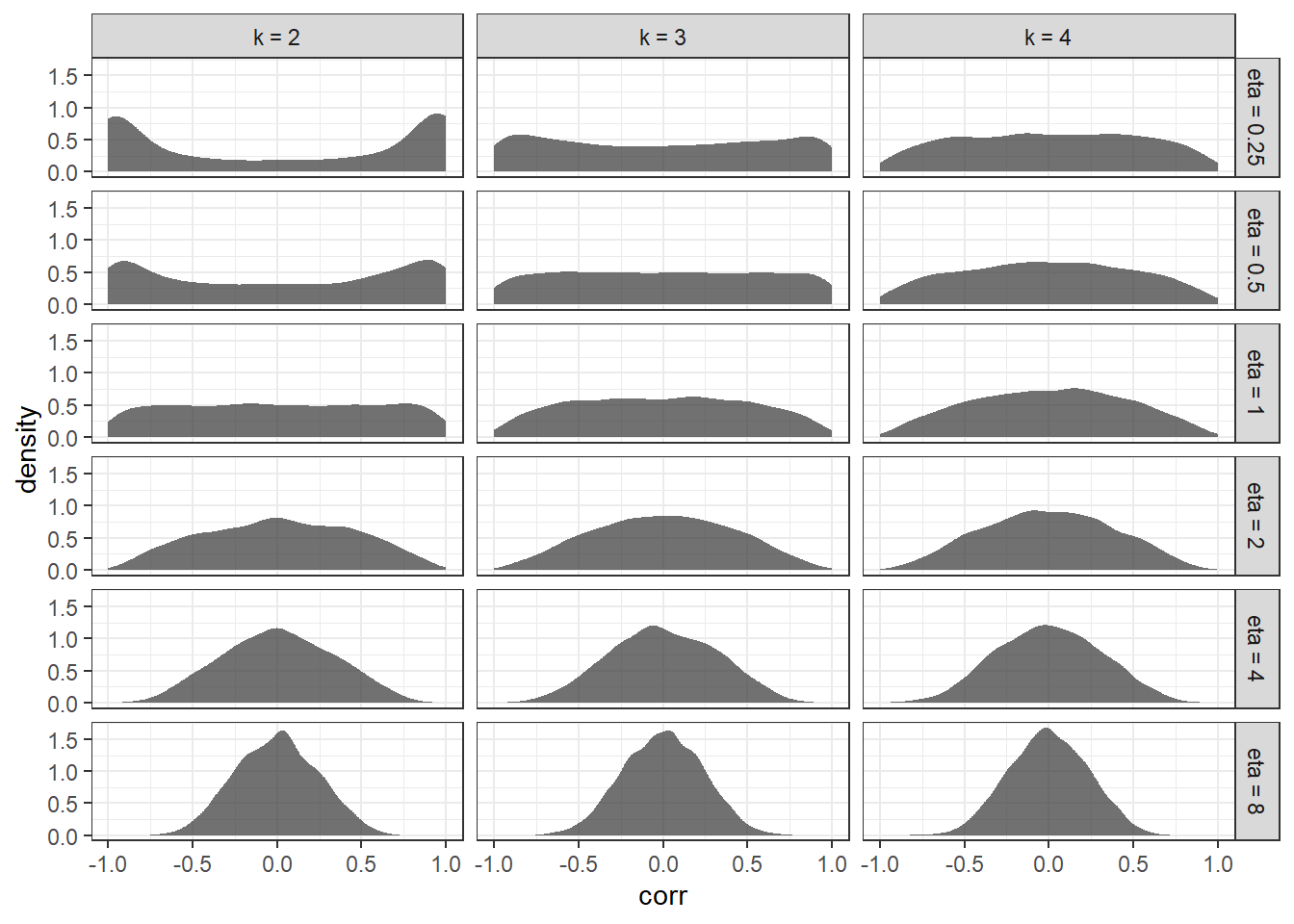
Figure 6.1: Simulated distributions of correlations from the LKJ distribution. \(k\) is the matrix size, and \(\eta\) is the parameter in the LKJ distribution.
Figure 6.1 confirms main features of the LKH distribution, as outlined in Section 1.13 of the Stan User’s Guide
The basic behavior of the LKJ correlation distribution is similar to that of a beta distribution. For \(\eta=1\), the result is a uniform distribution. Despite being the identity over correlation matrices, the marginal distribution over the entries in that matrix (i.e., the correlations) is not uniform between -1 and 1. Rather, it concentrates around zero as the dimensionality increases due to the complex constraints. For \(\eta>1\), the density increasingly concentrates mass around the unit matrix, i.e., favoring less correlation. For \(\eta<1\), it increasingly concentrates mass in the other direction, i.e., favoring more correlation.
That is, for small correlation matrices (say, \(k=2\)), the distribution is more spread out, and the modes are more pronounced when \(\eta<1\). Visually, it seems like the matrix size \(k\) is less important for larger values of \(\eta\). All of this is to say, we probably want to choose an \(\eta>1\) (which is also recommended by the Guide), but we will also want to choose \(\eta\) differently depending on the number of participant-level parameters \(k\) we have in our model.
Section 1.13 of the Stan User’s Guide24 also suggests using Cholesky factorization to further decompose the correlation matrix \(\Omega\). That is, we can represent \(\Omega\) as the outer product of a triangular matrix \(L_\Omega\) with itself:
\[ \Omega = L_\Omega L_\Omega^\top \]
This is particularly useful because we can then express our participant-level parameters as a linear combination of standard normal random variables:
\[ \begin{aligned} \theta_i&=\mu+\mathrm{diag}(\tau)L_\Omega z_i\\ z_{i,j}&\sim iid N(0,1) \end{aligned} \]
This representation speeds up computation because evaluating the multivariate normal density and the LKJ prior both require factorization. By re-parameterizing the model in terms of the already factorized values, we avoid this factorization. This also permits writing the whole collection of individual parameters \(\theta=(\theta_1,\theta_2,\ldots,\theta_n)\) as one big matrix operation involving the already factorized parameters, and standard normals (which are very fast to simulate):
\[ \begin{aligned} \theta&=\mu 1_n^\top+\mathrm{diag}(\tau)L_\Omega z \\ z_{j,i}&\sim iidN(0,1) \end{aligned} \]
where \(z\) is a \(k\times n\) matrix of standard normals.
All of these modifications might make your model less intuitive to read, but they will make it easier for Stan to simulate your posterior quickly and without errors. What we will end up with is a model whose actual parameters are \(\{\mu,\tau,L_\Omega,z\}\) instead of \(\{\mu,\Sigma,\theta\}\), however we will always be able to generate the (hopefully) more interpretable parameters of \(\Sigma\), \(\Omega\), and \(\theta\), because there is a deterministic relationship between them.
6.4.2 Transformed parameters and normal distributions
One restriction that applies when estimating a hierarchical model with a multivariate normal distribution of individual-level parameters is that these individual-level parameters must be able to take on any real number. This is not a problem for, say, the risk-aversion parameter \(r\) in the CRRA utility function \(u_i(x)=\frac{x^{1-r_i}}{1-r_i}\), however there are many other cases where our models’ parameters must be resrticted to only a subset of the real number line. For these parameters, we are going to have to transform them before they enter the model. That is, instead of estimating (say) logit choice precision parameter \(\lambda\), which must be positive, we could estimate \(\log\lambda\), as \(\log(\cdot)\) takes a positive real number, and maps it onto the real number line. Other times, our parameters need to be restricted to the unit interval. In these cases one can use the inverse logit (\(\log(x)-\log(1-x)\)) or inverse normal cumulative density \(\Phi^{-1}(x)\).
6.5 Example: again with Bruhin, Fehr, and Schunk (2019)
library(tidyverse)

d1<-(read.csv("Data/BFS2019_choices_exp1.csv")
     |> mutate(experiment=1)
)
d2<-(read.csv("Data/BFS2019_choices_exp2.csv")
     |> mutate(experiment=2)
)
D<-(rbind(d1,d2)
     # Just use the dictator game data
     |> filter(dg==1)
     |> mutate(
       self_alloc = ifelse(choice_x==1,self_x,self_y),
       other_alloc = ifelse(choice_x==1,other_x,other_y)
     )
)
I will begin with again analyzing the modified dictator game decisions in Bruhin, Fehr, and Schunk (2019), which I introduced in the previous chapter. Recall that in this experiment, 174 participants each made 78 pairwise choices over allocations of money between themself and another participant. As with the previous chapter, I will stick with the Fehr and Schmidt (1999) model of inequality-aversion as the deterministic economic model:
\[ U(\pi_1,\pi_2;\alpha_i,\beta_i)=\pi_1-\alpha_i\max\{\pi_2-\pi_1,0\}-\beta_i\max\{\pi_1-\pi_2\} \] and the logistic choice model to make it a probabilistic model that permits a likelihood representation:
\[ X_{i,t}\mid \theta,\mu,\Sigma\sim\mathrm{Bernoulli}\left(\Lambda\left(\lambda_i\left( U(\pi^X_1,\pi^X_2;\alpha_i,\beta_i)-U(\pi^Y_1,\pi^Y_2;\alpha_i,\beta_i) \right)\right)\right) \]
While this statement of the model is almost identical to how I made it in the previous chapter, there are some changes in notation that need to be noted. Firstly, I have explicitly put an \(i\) subscript on the individual-level parameters \(\alpha_i\), \(\beta_i\), and \(\lambda_i\). This is to make it clear that each participant \(i\) has their own parameters. For ease of notation here, I have lumped all of these parameters together into \(\theta\), so that we can talk about the population distribution more compactly. That is:
\[ \theta_i=\begin{pmatrix}\alpha_i&\beta_i&\log\lambda_i\end{pmatrix}^\top \] where taking the log of \(\lambda\) ensures that all elements of the (transformed) parameter vector \(\theta\) can take on any real number. The above sampling statement also conditions on the population level parameters \(\mu\) and \(\Sigma\), however we do not see any elements of these parameters on the right-hand side of the sampling statement. This is because it is assumed that \(\theta\), and in fact just \(\theta_i\), contains all of the information about the distribution of choices \(X_{i,t}\) for participant \(i\). Put differently, once we know a participant’s parameters \(\theta_i\), the population distribution does not tell us anything more about the distribution of their choices.
To fully specify the likelihood, we need to specify how the individual-level parameters \(\theta_i\) are generated by the population-level parameters \(\mu\) and \(\Sigma\). Let’s specify an independent multivariate normal distribution for \(\theta_i\):
\[ \theta_i\sim iid N(\mu,\Sigma) \] where \(\mu\) is the population mean of \(\theta_i\) and \(\Sigma\) is the population variance-covariance matrix of \(\theta_i\).
At this point, note that if I told you the population level parameters \(\mu\) and \(\Sigma\), then you would be able to simulate data from the experiment. Specifically, you would draw \(n\) \(\theta_i\)s from the multivariate normal, and then use these \(\theta_i\)s to simulate the binary choices \(\{X_{i,t}\}_{i=1,t=1}^{n,T}\). This means we have all of the information needed to specify the likelihood. What remains is to choose priors for the population-level parameters \(\mu\) and \(\Sigma\). As building up priors on variance-covariance matrices can be daunting if handled in one go, I will first take you through a model that assumes that the individual-level parameters are uncorrelated. Fortunately this for us, this is a really useful stepping stone for the correlated model, because Stan lets us decompose a variance-covariance matrix into a vector of standard deviations and a correlation matrix.
6.5.1 No correlation between individual-level parameters
Suppose to begin with that our individual-level parameters are not correlated with each other. We can therefore re-write the hierarchical structure of the model as:
\[ \begin{aligned} \theta_{i,\alpha}&\sim iid N(\mu_\alpha,\tau_\alpha^2)\\ \theta_{i,\beta}&\sim iid N(\mu_\beta,\tau_\beta^2)\\ \theta_{i,\lambda}&\sim iid N(\mu_\lambda,\tau_\lambda^2)\\ \end{aligned} \]
6.5.1.1 A quick prior calibration
Here it is appropriate to assign normal priors to the mean parameters, and half Cauchy priors (i.e. truncated to be positive only) to the standard deviations. As with the example using this dataset in the previous chapter, let’s start by selecting a prior for \(\lambda_i\). However this time, we need to specify priors for the parameters that govern the distribution of \(\lambda_i\). Here, I decided to use the following prior for \(\lambda\) in the representative agent model:
\[ \log\lambda\sim N(-5.76,2.11^2) \] It seems reasonable that we will want the prior mean of \(\mu_\lambda\) to be in the same location, so this leaves us with working out an appropriate prior standard deviation for \(\mu_\lambda\). Recall that in this previous example, I used the model’s predicted probability for a selfish participant as a gauge for where the economically interesting values of \(\lambda\) were. Again, we can then limit ourselves to looking at twelve different payoff differences:
d<-(D
    |> mutate(absDiff = abs(self_x-self_y))
    |> dplyr::select(absDiff)
    |> unique()
    )
d$absDiff |> print()
## [1] 140 200 380 240 120 80 40 280 180 0 160 360As this problem will be a bit more complicated, I will just focus on the median value of these differences:
## [1] 170Furthermore, since we are taking the log of \(\lambda\), \(\exp(\mu_\lambda)\) gives us the median of the distribution of the predicted choice probability. Figure 6.2 shows how the distribution of this choice probability, summarized by the median, 2.5th, 25th, 75th, and 97.5th percentiles, changes as we change the prior standard deviation of \(\mu_\lambda\). Here, we don’t want to set the prior standard deviation too small, because otherwise it would influence our posterior too much. On the the other hand, we don’t want to set it too large, either, because this could mean we are searching for solutions of our model in unlikely regions of the parameter space. For me, choosing a prior standard deviation of one find this happy middle ground. That is, I will go with:
\[ \mu_\lambda\sim N(-5.76,1^2) \]
lambdaCheck<-(
  tibble(priorSD = seq(0,4,length=100))
      |> mutate(
        PrMedian = 1/(1+exp(-exp(-5.76)*dMedian)),
        Pr975    = 1/(1+exp(-exp(-5.76+priorSD*1.96)*dMedian)),
        Pr025    = 1/(1+exp(-exp(-5.76-priorSD*1.96)*dMedian)),
        Pr750    = 1/(1+exp(-exp(-5.76+priorSD*0.67)*dMedian)),
        Pr250    = 1/(1+exp(-exp(-5.76-priorSD*0.67)*dMedian)),
        )
)

(
  ggplot(lambdaCheck,aes(x=priorSD,y=PrMedian))
  +geom_path()
  +geom_ribbon(aes(ymax=Pr975,ymin=Pr025),alpha=0.2)
  +geom_ribbon(aes(ymax=Pr750,ymin=Pr250),alpha=0.4)
  +theme_bw()
  +ylab("median probability of choosing the option with the greatest utility")
  +xlab("prior standard deviation of the population mean parameter for \u03bb")
)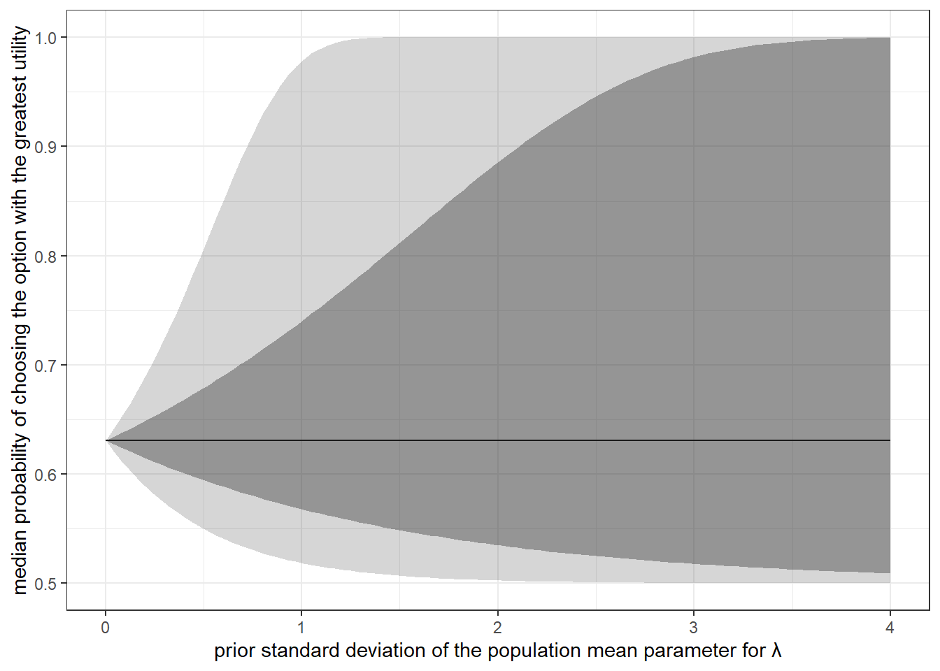
Figure 6.2: A plot of the distribution of predicted choice probabilities that will help us calibrate the priors for choice precision.
Figure 6.2 will also be helpful to us in choosing a prior for \(\tau_\lambda\), the standard deviation of \(\log\lambda_i\). Firstly, since I have limited myself to priors of the form:
\[ \tau_\lambda\sim \mathrm{Cauchy}^+(0,g) \]
it is informative to know that the cumulative distribution function of \(\tau_\lambda\) is:
\[ \begin{aligned} F(x)&=\frac{2}{\pi}\mathrm{arctan}\left(\frac{x}{g}\right)I(x\geq0) \end{aligned} \] and so we can write the inverse cumulative density function as:
\[ F^{-1}(p)=g\tan \left(\frac{\pi p}{2}\right) \]
so the 95th percentile of the distribution is \(F^{-1}(0.95)=g\tan(0.95\pi/2)\approx 12.7g\). Figure 6.2 shows us, if we fix \(\mu_\lambda\) to its prior median of \(-5.76\), what the implications of different values of \(\tau_\lambda\) are. That is, we can re-label the horizontal axis as “\(\tau_\lambda\)”, and the vertical axis as “distribution of choice probabilities if \(\mu_\lambda=-5.76\)”. Since for \(\tau_\lambda>3\) the interquartile range of the distribution of this choice probability (dark shaded region) takes up almost all of the vertical distance, these seem like unlikely values. Therefore I will calibrate the prior so \(\tau_\lambda=3\) is the 95th percentile of its distribution. Therefore \(g=3/12.7\approx0.24\), so:
\[ \begin{aligned} \mu_\lambda&\sim N(-5.76,1^2)\\ \tau_\lambda&\sim \mathrm{Cauchy}^+(0,0.24) \end{aligned} \]
For the priors for the parameters governing the distributions of \(\alpha_i\) and \(\beta_i\), I will keep them centered on zero. This means that I am looking to fill the blanks in the following distributions:
\[ \mu_\alpha\sim N(0,s^2),\quad \tau_\alpha\sim \mathrm{Cauchy}^+(0,g) \] and similarly for \(\mu_\beta\), and \(\tau_\beta\). While in the representative agent model I calibrated the priors for \(\alpha\) and \(\beta\) so that 75% of the prior distribution was in the range \((-1,1)\), this would put too much mass outside this region for their population means: we should expect there to be less prior uncertainty in \(\mu_\alpha\) than in \(\alpha\). This is because \(\mu_\alpha\) is a measure of central tendency for \(\alpha_i\), and so it seems reasonable that prior to observing the data, we should be more certain about \(\mu_\alpha\) than an individual \(\alpha_i\). Therefore, I will calibrate the priors for \(\mu_\alpha\) and \(\mu_\beta\) so that 99% of the probability mass is in this region, so \(s=2.58^{-1}\approx0.39\). For \(g\), a standard deviation of one seems large to me for both \(\alpha\) and \(\beta\), because these parameters being greater than one means that the participant will place more weight on the other person’s earnings than their own. Choosing \(g=0.079\) means that having \(\tau_\alpha>1\) will happen only 5% of the time in the prior. Therefore, all together my priors for this model are:
\[ \begin{aligned} \mu_\alpha&\sim N(0,0.39^2),\quad \tau_\alpha\sim \mathrm{Cauchy}^+(0,0.79)\\ \mu_\beta&\sim N(0,0.39^2),\quad \tau_\beta\sim \mathrm{Cauchy}^+(0,0.79)\\ \mu_\lambda&\sim N(-5.76,1^2),\quad \tau_\lambda\sim\mathrm{Cauchy}^+(0,0.24) \end{aligned} \]
6.5.1.2 Implementation and estimation in Stan
This is where all of the work we did in making the representative agent model comes in handy. Here is all we have to do:
- Add in another data variable that keeps track of the participant id (i.e. the \(i\) index)
- Change the prior data variables so that they are for priors over the population-level parameters
- Modify the existing parameters in the parameters block so that they are participant-specific
- Add in the new population-level parameters in the parameters block
- Specify the hierarchical structure in the model block
This might seem like a lot, but it will be exactly the same every time we make a model hierarchical. Importantly, we barely have to modify any of the part of the code that does the individual-level likelihood parts. Here is what I came up with after unashamedly copying and pasting my representative agent model code into a new file:25
data {
  int<lower=0> n; // number of observations
  vector[n] self_x; // payoff to self with allocation x
  vector[n] other_x; // payoff to other with allocation x
  vector[n] self_y; // payoff to self with allocation y
  vector[n] other_y; // payoff to other with allocation y
  int choice_x[n]; // =1 iff allocation x is chosen

  /* <----- ADDITION: we need a variable to keep track of the participant ids
  We also need an integer telling us how many participants we have
  */
  int id[n];
  int nParticipants;

  /* <---- DELETION: we now have priors over population-level parameters
  real prior_lambda[2];
  real prior_alpha[2];
  real prior_beta[2];
  */

  // <---- ADDITION: data specifying the priors;
  real prior_mu_alpha[2];
  real prior_mu_beta[2];
  real prior_mu_lambda[2];
  real prior_tau_alpha;
  real prior_tau_beta;
  real prior_tau_lambda;

}

transformed data {
  vector[n] dX; // disadvantageous inequality at allocation x
  vector[n] dY; // disadvantageous inequality at allocation y
  vector[n] aX; // advantageous inequality at allocation X
  vector[n] aY; // advantageous inequality at allocation X

  dX = fmax(0,other_x-self_x);
  dY = fmax(0,other_y-self_y);
  aX = fmax(0,self_x-other_x);
  aY = fmax(0,self_y-other_y);
}
parameters {

  /* <--- MODIFICATION: the individual-level parameters are now vectors
  */
  vector[nParticipants] alpha;
  vector[nParticipants] beta;
  vector<lower=0>[nParticipants] lambda;

  // <---- ADDITION: New population-level parameters
  real mu_alpha;
  real mu_beta;
  real mu_lambda;
  real<lower=0> tau_alpha;
  real<lower=0> tau_beta;
  real<lower=0> tau_lambda;


}
model {

  vector[n] Ux; // utility of allocation x
  vector[n] Uy; // utility of allocation y

  /* <---- MODIFICATION: Since the individual level parameters are now vectors,
  we need to adjust the utility equations so the right parameters are matched
  with the right observations. This is where the new id variable comes in
  */
  Ux = self_x-alpha[id] .* dX-beta[id] .* aX;
  Uy = self_y-alpha[id] .* dY-beta[id] .* aY;

  // <---- Slight modification to the likelihood to bring in the id variable
  choice_x ~ bernoulli_logit(lambda[id] .* (Ux-Uy));

  /* <---- MODIFICATION: priors on individual level parameters are now
  statements about their relationship with population level parameters
  */
  alpha~normal(mu_alpha,tau_alpha);
  beta ~normal(mu_beta,tau_beta);
  lambda ~ lognormal(mu_lambda,tau_lambda);

  // <---- ADDITION: priors for population-level parameters
  mu_alpha ~ normal(prior_mu_alpha[1],prior_mu_alpha[2]);
  mu_beta ~ normal(prior_mu_beta[1],prior_mu_beta[2]);
  mu_lambda ~ normal(prior_mu_lambda[1],prior_mu_lambda[2]);

  tau_alpha ~ cauchy(0,prior_tau_alpha);
  tau_beta ~ cauchy(0,prior_tau_beta);
  tau_lambda ~ cauchy(0,prior_tau_lambda);

}
From here, we can pass the data to Stan and estimate the model:
file<-"Hierarchical/Hierarchical_BFS2019"

# Generate the id variable
D <-(
  D
  |> mutate(id = sid %>% paste() %>% as.factor() %>% as.numeric())
)
# only run if I haven't estimated it yet
if (!file.exists(paste0("Outputs/",file,"_independent.rds"))) {

  dStan<-list(
    n=dim(D)[1],
    self_x=D$self_x,
    other_x=D$other_x,
    self_y=D$self_y,
    other_y=D$other_y,
    choice_x=D$choice_x,

    id = D$id,
    nParticipants = D$id |> unique() |> length(),

    prior_mu_alpha   = c(0,0.39),
    prior_mu_beta    = c(0,0.39),
    prior_mu_lambda  = c(-5.76,1),
    prior_tau_alpha  = 0.79,
    prior_tau_beta   = 0.79,
    prior_tau_lambda = 0.24

  )
  Fit<-stan(paste0("Code/",file,"_independent.stan"),
            data=dStan,
            seed=42)
  saveRDS(Fit,paste0("Outputs/",file,"_independent.rds"))
}

Fit<-readRDS(paste0("Outputs/",file,"_independent.rds"))

# rstan::summary(Fit)$summary |> View()
Interestingly (to me at least), this one did not take as long as I expected (under ten minutes on my laptop). This is compared to about half an hour for the individual-specific estimations in the previous chapter. Think about this: even though we estimated \(3n\) parameters in the individual-specific estimations, and \(3n+6\) parameters just now, the second estimation was faster! While I don’t have a well-thought-out explanation for this, my intuition is that the population-level parameters are forming a much more informative “prior” over the individual-level parameters, so sampling the individual-level parameters is less burdensome for Stan.
Anyway, we may as well look at the estimates. As we have so many individual-level parameters, I will just show a summary in Table 6.1 for the population-level parameters:
s<-rstan::summary(Fit)$summary

# identify the rows that contain the population-level parameters.
# These have row names that contain the character "_"
II<- grepl("_",rownames(s))
s[II,] |> kbl(digits=3,caption="Population estimates of a model assuming a hierarchical independent distribution of individual-level parameters.") |>
kable_classic(full_width=FALSE)| mean | se_mean | sd | 2.5% | 25% | 50% | 75% | 97.5% | n_eff | Rhat | |
|---|---|---|---|---|---|---|---|---|---|---|
| mu_alpha | -0.030 | 0.000 | 0.014 | -0.058 | -0.040 | -0.030 | -0.020 | -0.001 | 3933.694 | 0.999 |
| mu_beta | 0.233 | 0.000 | 0.020 | 0.195 | 0.219 | 0.233 | 0.246 | 0.271 | 6327.612 | 0.999 |
| mu_lambda | -3.498 | 0.001 | 0.072 | -3.636 | -3.546 | -3.499 | -3.450 | -3.353 | 3126.904 | 1.001 |
| tau_alpha | 0.165 | 0.000 | 0.015 | 0.138 | 0.155 | 0.165 | 0.175 | 0.196 | 2065.354 | 1.000 |
| tau_beta | 0.248 | 0.000 | 0.016 | 0.219 | 0.237 | 0.247 | 0.259 | 0.283 | 4071.073 | 1.001 |
| tau_lambda | 0.829 | 0.001 | 0.066 | 0.708 | 0.784 | 0.827 | 0.871 | 0.971 | 2094.545 | 1.002 |
| lp__ | -2345.289 | 0.439 | 16.981 | -2379.805 | -2356.544 | -2345.241 | -2333.389 | -2312.640 | 1493.791 | 1.000 |
6.5.2 Correlation between individual-level parameters
Now let’s modify the model so that we can estimate a correlation matrix for our participant-level parameters. Conceptually, this is a fairly straightforward step, as we have already assigned priors to \(\mu\) and \(\tau\): by decomposing \(\Sigma\) into \(\tau\) and \(\Omega\), really the only bit of thinking we need to do is to assign an appropriate prior for \(\Omega\). For this, I choose:
\[ \Omega\sim \mathrm{LKJCorr}(2) \] which seems like a reasonably spread-out but still unimodal distribution, as shown in Figure 6.1 for \(k=3\) participant-level parameters. Here is what I came up with for the code for the hierarchical model with correlated parameters.
data {
  int<lower=0> n; // number of observations
  vector[n] self_x; // payoff to self with allocation x
  vector[n] other_x; // payoff to other with allocation x
  vector[n] self_y; // payoff to self with allocation y
  vector[n] other_y; // payoff to other with allocation y
  int choice_x[n]; // =1 iff allocation x is chosen

  int id[n];
  int nParticipants;


  vector[2] prior_mu[3];
  real prior_tau[3];
  real prior_LKJ;

  // number of simulation steps to approximate demand
  int nsim;
  // Endowment of tokens for demand
  int W;
  // number of prices to evaluate demand at
  int nrho;
  // prices to evaluate demand at
  vector[nrho] rho;


}

transformed data {
  vector[n] dX; // disadvantageous inequality at allocation x
  vector[n] dY; // disadvantageous inequality at allocation y
  vector[n] aX; // advantageous inequality at allocation X
  vector[n] aY; // advantageous inequality at allocation X

  dX = fmax(0,other_x-self_x);
  dY = fmax(0,other_y-self_y);
  aX = fmax(0,self_x-other_x);
  aY = fmax(0,self_y-other_y);

  // some things used to produce demand
  vector[W+1] X;
    for (xx in 1:(W+1)) {
      X[xx] = xx-1;
    }


}
parameters {

  vector[3] mu; // population mean
  vector<lower=0>[3] tau; // population standard deviation
  cholesky_factor_corr[3] L_Omega; // Cholesky factorization of the correlation matrix

  matrix[3,nParticipants] z; // standard normals determinig participants' parameters

}
model {

  vector[n] Ux; // utility of allocation x
  vector[n] Uy; // utility of allocation y
  vector[n] alpha;
  vector[n] beta;
  vector[n] lambda;

  matrix[3,nParticipants] theta;

  theta = mu*rep_row_vector(1.0,nParticipants)
                    +diag_pre_multiply(tau,L_Omega)*z;

  alpha  = theta[1,id]';
  beta   = theta[2,id]';
  lambda = exp(theta[3,id]');

  Ux = self_x-alpha .* dX-beta .* aX;
  Uy = self_y-alpha .* dY-beta .* aY;

  choice_x ~ bernoulli_logit(lambda .* (Ux-Uy));

  to_vector(z) ~ std_normal();

  for (pp in 1:3) {
    mu[pp] ~ normal(prior_mu[pp][1],prior_mu[pp][2]);
    tau[pp] ~ cauchy(0.0,prior_tau[pp]);
  }

   L_Omega ~ lkj_corr_cholesky(prior_LKJ);
}

generated quantities {
  matrix[3,3] Omega;
  matrix[3,nParticipants] theta;
  theta = mu*rep_row_vector(1.0,nParticipants)
                    +diag_pre_multiply(tau,L_Omega)*z;
  Omega = L_Omega*L_Omega';

  // store demand in this vector
  vector[nrho] demand;

  {
    // simulated standard normals
    matrix[3,nsim] zsim;
    for (rr in 1:3) {
      zsim[rr,] = to_row_vector(normal_rng(rep_vector(0.0,nsim),rep_vector(1.0,nsim)));
    }

    // simulate parameters
    matrix[3,nsim] thetasim;
    thetasim = mu*rep_row_vector(1.0,nsim)
                    +diag_pre_multiply(tau,L_Omega)*zsim;

    vector[nsim] alphasim = thetasim[1,]';
    vector[nsim] betasim = thetasim[2,]';
    vector[nsim] lambdasim = exp(thetasim[3,]');

    // go through each value of rho
    for (rr in 1:nrho) {

      // dump individual-level expected demand in here
      vector[nsim] Y;
      for (ss in 1:nsim) {

        // utility of choosing each allocation
        vector[W+1] U = X
            -alphasim[ss]*fmax(0.0,(W-X*(1.0+rho[rr]))/rho[rr])
            -betasim[ss]*fmax(0.0,(X*(1+rho[rr])-W)/rho[rr]);
        // probability of choosing each allocation
        vector[W+1] pr = softmax(lambdasim[ss]*U);
        // expected tokens kept
        real EX = sum(X.*pr);
        // expected tokens bought for the other participant
        Y[ss] = (W-EX)/rho[rr];

      }

      demand[rr] = mean(Y);

    }


  }


}
Here I am implementing both the Cholesky decomposition of \(\Omega\) and the vectorization as described in Section 1.13 of the Stan User’s Guide. In particular, note that \(\theta\) is not declared in the parameters block. Rather, I use the matrix z of standard normals to generate \(\theta\) in the model block:
Also, since \(\Omega\) is not a fundamental parameter, I generate it in the generated quantities block so that we can look at it later.
Here’s how you estimate the model in RStan:26
library(rstan)
rstan_options(auto_write = TRUE)
options(mc.cores = parallel::detectCores())

if (!file.exists(paste0("Outputs/",file,"_correlated.rds"))) {

  dStan<-list(
    n=dim(D)[1],
    self_x=D$self_x,
    other_x=D$other_x,
    self_y=D$self_y,
    other_y=D$other_y,
    choice_x=D$choice_x,

    id = D$id,
    nParticipants = D$id |> unique() |> length(),

    prior_mu = rbind(c(0,0.39),
                     c(0,0.39),
                     c(-5.76,1)
                     ),
    prior_tau = c(0.79,0.79,0.24),
    prior_LKJ = 2,

    # data needed for demand calculation
    # (see the "Doing something with the estimates" section)
    nsim=100,
    W = 1000,
    nrho = 100,
    rho = seq(0.1,10,by=0.1)


  )
  Fit<-stan(paste0("Code/",file,"_correlated.stan"),
            data=dStan,
            seed=42)
  saveRDS(Fit,paste0("Outputs/",file,"_correlated.rds"))
}

Fit<-readRDS(paste0("Outputs/",file,"_correlated.rds"))
There are quite a lot of parameters in this model (because we are using data augmentation), so looking at the entire summary is somewhat daunting and not particularly useful. Fortunately, I set up the parameters block so that the first six parameters listed have the same interpretation as the model in the previous section that assumes no correlation between parameters (except that we are estimating \(\lambda\) as \(\log\lambda\)):
summary(Fit)$summary[1:6,] |> kbl(caption = "Posterior estimates from the model with correlated parameters.",digits=3) |> kable_classic(full_width=F)| mean | se_mean | sd | 2.5% | 25% | 50% | 75% | 97.5% | n_eff | Rhat | |
|---|---|---|---|---|---|---|---|---|---|---|
| mu[1] | -0.014 | 0.001 | 0.015 | -0.044 | -0.024 | -0.014 | -0.004 | 0.017 | 898.269 | 1.008 |
| mu[2] | 0.230 | 0.001 | 0.020 | 0.191 | 0.216 | 0.230 | 0.243 | 0.269 | 1156.227 | 1.004 |
| mu[3] | -3.531 | 0.002 | 0.068 | -3.662 | -3.576 | -3.532 | -3.486 | -3.394 | 1593.340 | 1.004 |
| tau[1] | 0.175 | 0.000 | 0.014 | 0.149 | 0.165 | 0.174 | 0.184 | 0.204 | 1584.464 | 1.001 |
| tau[2] | 0.242 | 0.000 | 0.016 | 0.211 | 0.231 | 0.241 | 0.252 | 0.275 | 1692.600 | 1.000 |
| tau[3] | 0.774 | 0.002 | 0.062 | 0.660 | 0.731 | 0.771 | 0.814 | 0.902 | 1292.542 | 1.001 |
To read Table 6.2, recall that the order of parameters in the vectors \(\mu\) and \(\tau\) is \((\alpha_i\ ,\beta_i\ ,\ \log\lambda_i)^\top\). These population-level parameters are all quite similar to those estimated in the previous section, where we assumed no correlation between the participant-level parameters. However now we also get estimates of the correlations between these parameters, which can be see in tin Table 6.3. In particular, note the strong negative correlation between \(\alpha\) and \(\beta\): this is something we would not have beed able to comment on had we just estimated the model without correlation.
Omega<-extract(Fit)$Omega

OmegaMean<-Omega |> apply(c(2,3),mean)
OmegaSD  <-Omega |> apply(c(2,3),sd)

table<-paste0(OmegaMean |> round(3),
              "  (",OmegaSD |> round(3),")") |> matrix(nrow=3)

colnames(table)<-c("$\\alpha$","$\\beta$","$\\log\\lambda$")
rownames(table)<-c("$\\alpha$","$\\beta$","$\\log\\lambda$")

table|> kbl(digits=3,caption = "Estimated correlation matrix $\\Omega$. Posterior means shown with posterior standard deviations in parentheses.") |>
kable_classic(full_width=FALSE)| \(\alpha\) | \(\beta\) | \(\log\lambda\) | |
|---|---|---|---|
| \(\alpha\) | 1 (0) | -0.689 (0.061) | -0.594 (0.064) |
| \(\beta\) | -0.689 (0.061) | 1 (0) | -0.005 (0.088) |
| \(\log\lambda\) | -0.594 (0.064) | -0.005 (0.088) | 1 (0) |
Finally, let’s have a look at the model’s shrinkage estimates. Recall that these come from the data-augmentation process, and can be thought of as participant-specific estimates, had we used the parameters \(\mu\) and \(\Sigma\) that we estimated as our prior for these parameters. As with the previous chapter, I will focus on parameters \(\alpha\) and \(\beta\), which are the parameters of the Fehr and Schmidt (1999) inequality-aversion model. Also, as with the previous chapter, I will just plot their posterior means to avoid over-plotting. I show these in Figure 6.3
# extract the right parameters from the Stan Fit object
# and take the mean
theta<-extract(Fit)$theta |> apply(c(2,3),mean)|> t()
dTheta<-tibble(alpha=theta[,1],beta=theta[,2],lambda = exp(theta[,3]))

regions<-tibble(
  alpha = c(0.25,-0.25,-0.25,0.25),
  beta = c(0.5,-0.5,0.8,-0.5),
  label = c("inequality averse",
            "inequality loving",
            "efficiency loving",
            "competitive"
            )
)

(
  ggplot(
    data = dTheta,
    aes(x=alpha,y=beta,color=log(lambda))
  )
  +geom_point()
  +geom_text(data=regions,aes(x=alpha,y=beta,label=label),color="black")
  +theme_bw()
  +xlab(expression(alpha))+ylab(expression(beta))
  +geom_hline(yintercept=0,linetype="dashed")
  +geom_vline(xintercept=0,linetype="dashed")
)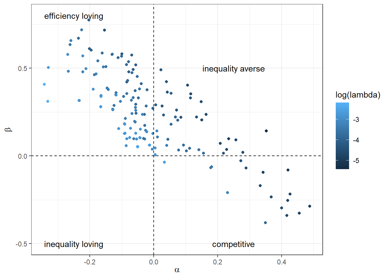
Figure 6.3: Posterior mean estimates of individual-level parameters \(\alpha\) and \(\beta\) from the hierarchical model assuming correlation between the parameters.
6.5.2.1 Doing something with the estimates
Now that we have a model and estimates that respect the heterogeneity we believe is present in the population, how about we use it to make an out-of-sample prediction? For this exercise, we will use the estimated model to predict a demand curve for charitable giving, a la Andreoni and Vesterlund (2001) and Andreoni and Miller (2002). To do this, suppose that a participant has 1000 tokens,27 which she can either keep, or use to buy income for another participant, who starts out with nothing. Kept tokens generate income of 1 experimental currency unit for the participant, and the participant can buy 1 experimental currency unit for the other participant for a price of \(\rho\). Therefore, if \(x\) is the income of the participant, and \(y\) is the income of the other, then the budget constraint is:
\[ \begin{aligned} 1000 = x+\rho y \end{aligned} \]
The participant’s utility function is then:
\[ \begin{aligned} U_i(x,y)=x-\alpha_i\max\{0,y-x\}-\beta\max\{0,x-y\} \end{aligned} \]
And substituting the budget constraint into the utility function yields utility just as a function of \(x\):
\[ \begin{aligned} U_i(x)&=x-\alpha_i\max\left\{0,\frac{1000-x}{\rho}-x\right\}-\beta_i\max\left\{0,x-\frac{1000-x}{\rho}\right\}\\ U_i(x)&=x-\alpha_i\max\left\{0,\frac{1000-x(1+\rho)}{\rho}\right\}-\beta_i\max\left\{0,\frac{x(1+\rho)-1000}{\rho}\right\} \end{aligned} \]
Now assume that participants use logit choice with the same \(\lambda_i\) as in the original experiment.28 So the distribution of choices given \((\alpha_i,\beta_i,\lambda_i)\) is:
\[ \Pr(X = x\mid \alpha_i,\beta_i,\lambda_i,\rho)=\frac{\exp(\lambda_i U_i(x))}{\sum_{k=0}^{1000}\exp(\lambda_iU_i(k))} \]
So:
\[ E[X\mid \alpha_i,\beta_i,\lambda_i,\rho]=\frac{\sum_{x=0}^{1000}x\exp(\lambda_i U_i(x))}{\sum_{k=0}^{1000}\exp(\lambda_iU_i(k))} \]
But what we really want to report is the demand for giving to the other participant, so we need to convert this into income bought for the other participant (\(y\)):
\[ E[Y\mid \alpha_i,\beta_i,\lambda_i,\rho] = \frac{1000-E[X\mid \alpha_i,\beta_i,\lambda_i,\rho]}{\rho} \]
This is participant \(i\)’s (average, since they use probabilistic choice) demand for giving. But what we really want is a sense of what the population would demand. Hence, we need to integrate out the individual-specific parameters \(\alpha_i\), \(\beta_i\), and \(\lambda_i\). Mathematically, we can apply the law of iterated expectations like this, where the left-hand side is what we want to report as a function of \(\rho\):
\[ E[Y\mid \rho]=E\left[E[Y\mid \alpha_i,\beta_i,\lambda_i,\rho]\mid \rho\right] \]
In practice, this is a really hard expectation to take analytically, so instead we will do it with Monte Carlo integration:
\[ \begin{aligned} E[Y\mid \rho]&\approx \frac1S\sum_{s=1}^SE[Y\mid \alpha_s,\beta_s,\lambda_s,\rho]\\ \begin{pmatrix} \alpha_s\\ \beta_s \\ \log\lambda_s \end{pmatrix}&\sim iid N(\mu,\Sigma) \end{aligned} \]
You can see the implementation of this in the Stan file above. In particular, see the generated quantities block. In general, it is a good idea to use the generated quantities block to compute transformations of the parameters like this, as opposed to doing this outside of Stan in post-estimation. This is for at least two reasons. Firstly, since Stan is fast, this is probably the fastest way for you to compute things. Secondly, Stan gives you all of the convergence diagnostics for these transformed quantities, so you don’t need to worry about (say) having too small an effective sample size or a bad \(\hat R\) for these quantities.29
Now we can have a look at our estimated demand curve in Figure 6.4. For perspective, I also include the demand curve if participants chose allocations that equalized payoffs. This is shown with the red dashed line. Here we can see that participants are generally less generous than this, but get more generous than this for very low prices.
demand<-summary(Fit)$summary |>
  data.frame() |>
  rownames_to_column(var = "parameter") |>
  filter(grepl("demand",parameter)) |>
  mutate(
    price = seq(0.1,10,by=0.1),
    equal_split = 1000/(1+price)
  )

(
  ggplot(demand,aes(x=mean,y=price))
  +geom_line()
  +geom_line(aes(x=equal_split,y=price),color="red",linetype="dashed")
  +geom_ribbon(aes(xmin = X2.5.,xmax=X97.5.,y=price),alpha=0.5)
  +coord_cartesian(xlim = c(0,1500))
  +theme_bw()
  +ylab(expression("Price ("*rho*")"))
  +xlab("Quantity of experimental currency units demanded for the other participant")
)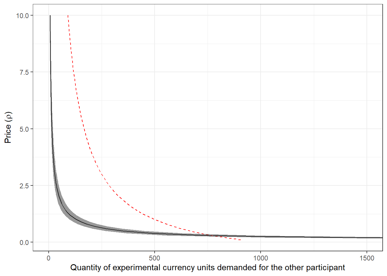
Figure 6.4: Estimted demand curve for giving. Line shows posterior mean estimate, shaded region shows a 95% Bayesian credible region (2.5th-97.5th percentile). Note that since this is a demand curve, the uncertainty is in the horizontal coordinates. Dashed red line shows the demand curve if participants equalized payoffs
Note that here we are making an out-of-sample prediction. That is, we are using our parameter estimates to predict how different participants (but drawn from the same population) would behave in a different environment (i.e. the budget set problem, rather than the binary choice task). This is a testable prediction if we run another experiment!
References
I.e. \(p(A,B)=p(A\mid B)p(B)\)↩︎
In fact, sometimes these are also referred to as “priors” in discussion of hierarchical models. I like to stay away from this language, as \(\mu\) and \(\Sigma\) are parameters that we are trying to estimate, rather than parameters describing our prior beliefs about other parameters.↩︎
This is a really useful section. I have it open in my browser most of the time that I am coding hierarchical models in Stan.↩︎
Here I have deliberately tried to leave as much of this Stan file as unchanged as possible so you can compare it side-by-side with the representative agent model. There are better ways to do this, which I will get to shortly. Most of them take advantage of the stacked vector \(\theta\) notation that I have used above.↩︎
This one will take a while. Fold some laundry, write some poetry, find Kakariko Village, or something. (about 17 minutes on my laptop)↩︎
I use 1000 tokens to keep the payoff scales similar to the original experiment.↩︎
This is a somewhat corageous assumption, as in the original experiment participants chose between two things at a time, and now we are asking them to choose between 1,001 things. ↩︎
I thank Brian Monroe for this insight.↩︎