4 Considerations for choosing a prior

Conceptually, the Bayesian techniques I am teaching you in the book are very similar to how we would approach the same inferential goals using maximum likelihood estimation.¹⁰ Both work with a likelihood function that specifies the distribution of data given the model’s parameters. The big difference between the two is that when using Bayesian techniques, we also need to specify a prior. That is, the likelihood is our formal statement about how our model’s parameters and the experiment generate data, and the prior is our formal statement about how much uncertainty we have about our model’s parameters before running an experiment. Whether we have had a good hard think about the prior we want to use, whether we have just thrown up our hands and gone for an improper “uninformative” flat prior, or anything in between, these are modeling choices. We should therefore pay at least some attention to our priors, and how they affect our estimates. This is especially the case for economic experiments, where sample sizes can be relatively small, and so the prior may still have substantial influence over the posterior.

We can assess our priors in several ways. If we want to take a stand on priors representing our actual prior beliefs about the uncertainty in our parameters, we can calibrate our priors using our expert knowledge of what reasonable and unreasonable parameter values are. For example, this could include choosing distributions that pin down what we think are reasonable 5% and 95% lower and upper bounds on the parameters.¹¹ We can also scrutinize our priors on parameters to check that they say about behavior. For example, we may check to see whether our calibrated prior makes reasonable predictions for behavior in the experiment. This might be useful if we are very uncertain about what reasonable values of our parameters are, but we have a better idea of what behavior might look like. Additionally, we can assess our prior’s performance in recovering the parameters of the model. That is, is there a prior that results in an estimator with better sampling properties than other choices?

A prior is useful not just in the estimation stage of our research, but also in the design stage. Priors can be immensely useful for tuning an experiment to best estimate our parameters of interest. A prior that actually reflects what we believe are plausible parameter values can help us choose experimental conditions that are the most informative of these parameters. This chapter is focused on ways for us to select a prior, not how to use it to design an experiment. I will devote a chapter to this at some point.

4.1 Example model and experiment

For this chapter I will use as an example the modified dictator game part of Bruhin, Fehr, and Schunk (2019), where participants made 78 pairwise choices of allocations between themselves and another participant. For this chapter, we will focus on estimating a simple one-parameter¹² other-regarding utility function:

\[ \begin{aligned} U(\pi_1,\pi_2,\alpha)&=\alpha\pi_1+(1-\alpha)\pi_2,\quad0\leq \alpha \leq 1 \end{aligned} \]

where $\pi_1$ and $\pi_2$ are the payoffs of the self and the other, respectively, and $\alpha\in[0,1]$ is the weight placed on the self’s payoff. Hence, $\alpha=1$ corresponds to self-regarding preferences. We will also assume a logit probabilistic choice rule with choice precision $\lambda>0$. Given the two allocations $(\pi_1^X,\pi_2^X)$ and $(\pi_1^Y,\pi_2^Y)$, we can write the likelihood as:

\[ \begin{aligned} p(y_t=1\mid \alpha,\lambda,\pi_t)&=\Lambda\left(\lambda\left(\alpha\pi_{t,1}^X+(1-\alpha)\pi_{t,2}^X-\alpha\pi_{t,1}^Y-(1-\alpha)\pi_{t,2}^Y\right)\right)\\ &=\Lambda\left(\lambda\left(\alpha(\pi_{t,1}^X-\pi_{t,1}^Y)+(1-\alpha)(\pi_{t,2}^X-\pi_{t,2}^Y)\right)\right) \end{aligned} \]

where $y_t=1$ iff allocation $X$ is chosen in decision $t$, zero otherwise. $\Lambda(x)=(1+\exp(-x))^{-1}$ is the inverse logit function.

The 78 pairwise choices in Bruhin, Fehr, and Schunk (2019) are shown in Figure 4.1. Each line segment represents a pairwise choice, with the coordinates of the endpoints showing the two allocations.

d1<-(read.csv("Data/BFS2019_choices_exp1.csv")
     |> mutate(experiment=1)
)
d2<-(read.csv("Data/BFS2019_choices_exp2.csv")
     |> mutate(experiment=2)    
)
D<-(rbind(d1,d2)
     # Just use the dictator game data
     |> filter(dg==1)  
     |> mutate(
       self_alloc = ifelse(choice_x==1,self_x,self_y),
       other_alloc = ifelse(choice_x==1,other_x,other_y)
     )
)

# We just need one participant's data because everything in this chapter will be simulation
BFS2019<-D |> filter(sid==102010050706)

(
  ggplot(
    BFS2019,
    
  )
  +geom_segment(aes(x=self_x,y=other_x,xend=self_y,yend=other_y))
  +theme_bw()
  +xlab("Own payoff")+ylab("Other's payoff")
  +geom_abline(slope=1,intercept=0,linetype="dashed")
  +coord_fixed()
)

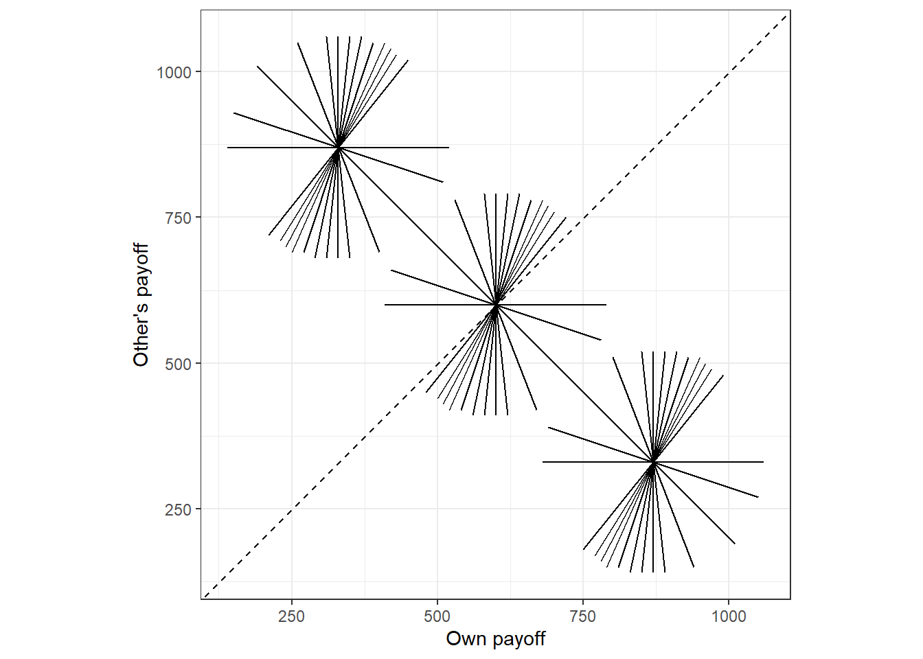
The 78 pairwise choices over allocations of money in the modified dictator game. Each pariwise choice is denoted by the endpoints of a line.

Figure 4.1: The 78 pairwise choices over allocations of money in the modified dictator game. Each pariwise choice is denoted by the endpoints of a line.

4.2 Getting the support right

To begin with, we need to choose which family of distributions we will use for our prior. This is where we rule out any nonsensical values, and make sure we do not rule out anything that could be reasonable. For example, if a parameter could in principle take on any real number, then a normal distribution makes sense. This allows us the freedom of choosing two properties of the prior distribution (the mean and standard deviation) to appropriately express our prior uncertainty in a parameter.

For the preference parameter $\alpha$, we have been given the restriction $\alpha\in[0,1]$, so here we need to choose a distribution that has a support of the unit interval. In this case, choosing something like the Beta distribution:

\[ \alpha\sim B(a_\alpha,b_\alpha) \]

the probit-normal distribution:

\[ \Phi^{-1}(\alpha)\sim N(m_\alpha,s_\alpha^2) \] or the logit-normal distribution:

\[ \log(\alpha)-\log(1-\alpha)\sim N(m_\alpha,s^2_\alpha) \]

could be reasonable choices, as they all permit us to independently choose two properties of the distribution. Furthermore, if the uniform distribution is something we would want to consider using, the Beta distribution (setting $a_\alpha=b_\alpha=1$) and the probit-normal distribution (setting $m_\alpha=0$, $s_\alpha=1$) nest this distribution, so these may be useful choices. For this example, I will choose the probit-normal distribution, as I use it quite commonly in my hierarchical models when I need to make this parameter restriction on an individual-level parameter.

For the choice precision parameter $\lambda$, we need to ensure that it is positive: negative values would imply that participants are less likely to choose the action with the greater utility, which is nonsensical. A good choice in this instance is the log-normal distribution. Again, this permits us to independently pin down two properties of the distribution.

\[ \log\lambda\sim N(m_\lambda,s^2_\lambda) \]

With the likelihood and the family of prior specified, we can go ahead and code this model up in Stan. This will be useful even before we have data, because we can use the Stan model to simulate data and explore the sampling properties of our estimator. Here you will see a few extras added to the model so we can do some more with it. In particular the UseData variable lets us turn the likelihood contribution on or off. That way we can get draws from both the prior and the posterior with the same model. Also, the UsePrior variable turns the prior on and off. This will enable us to see what happens when we use improper, flat, “uninformative” priors. It will also permit us to do maximum likelihood estimation.


// BFS2019priors.stan

data {
  int<lower=0> n; // number of decisions
  int y[n]; // choices. 1=X, 0=Y
  
  vector[n] self_x; // payoff to self with allocation x
  vector[n] other_x; // payoff to other with allocation x
  vector[n] self_y; // payoff to self with allocation y
  vector[n] other_y; // payoff to other with allocation y
  
  // priors
  real prior_lambda[2]; // log-normal
  real prior_alpha[2]; // probit-normal
  
  // Turns on and off whether we are using the data
  int<lower=0,upper=1> UseData; 
  
  // Turns on or off whether we are using the prior, or 
  // "uninformative" priors
  int<lower=0,upper=1> UsePrior;
}


parameters {
  real probitAlpha;
  real<lower=0> lambda;
}

transformed parameters {
  real<lower=0,upper=1> alpha = Phi(probitAlpha);
}


model {
  
  // priors
  if (UsePrior==1) {
    probitAlpha ~ normal(prior_alpha[1],prior_alpha[2]);
    lambda ~ lognormal(prior_lambda[1],prior_lambda[2]);
  }
  
  if (UseData==1) {
    y ~ bernoulli_logit(lambda*(
      alpha*(self_x-self_y)+(1-alpha)*(other_x-other_y)
       ));
  }
  
}

generated quantities {
  
  // predicted probability of choosing allocation X
  vector[n] probX = inv_logit(lambda*(
      alpha*(self_x-self_y)+(1-alpha)*(other_x-other_y)
       ));
  
  // Simulated data, 1 = chose allocation X
  int simX[n] = bernoulli_logit_rng(lambda*(
      alpha*(self_x-self_y)+(1-alpha)*(other_x-other_y)
       ));
  
}

4.3 Eliciting reasonable priors

As discussed in detail in Betancourt (2020) (Section 1.1), it is important for our models not to be built on assumptions that are in conflict with our “domain expertise”. That is as experts in the field, we may have a reasonable understanding of what are likely and unlikely parameter values before running an experiment, and we should incorporate this information into our prior. However translating a likely qualitative, general understanding of how participants might behave into a mathematical statement about the distribution of some parameters may not be straightforward. Two techniques Betancourt (2020) advocates for are the prior pushforward check, which checks whether our prior about a parameter is consistent with our understanding of our participants, and the prior predictive check, which checks whether our prior about a parameter is consistent with our understanding of our prior belief about summaries of the data that we might get. That is, a prior pushforward check is to check whether our chosen prior places too much, or not enough, mass in the wrong places of the parameter’s support, whereas the prior predictive check is to check whether our prior implies something implausible about summaries of our data (such as participants’ choices).

4.3.1 Parameter values and the prior pushforward check

Once we have settled on a family of distributions, perhaps the most direct way to hone in on the distribution within that family that we will actually use is by exploring the properties of these distributions. If we are just choosing a prior for a single (i.e. scalar) parameter, then we will most often have only a handful of degrees of freedom in our prior choice once we have selected a family of distributions. For example, the normal and beta families each allow us to independently pin down two properties of the distribution, while the exponential, Cauchy, and LKJ priors only allow for one. It is therefore very feasible to explore the properties of these distributions graphically.

d<-expand_grid(
  m = c(-0.4,0,0.4,0.8,1.2),
  s = c(0.25,0.5,1,2),
  sim = 1:10000
) |>
  rowwise() |>
  mutate(alpha = rnorm(1,mean=m,sd=s) |> pnorm()) |>
  ungroup() |>
  mutate(mtag = paste("m =",m),
         stag = paste("s =",s))

(
  ggplot(data=d,aes(x=alpha))
  +geom_histogram(bins=40)
  +facet_grid(stag~mtag)
  +theme_bw()
  +xlab(expression(alpha))
  +scale_x_continuous(n.breaks=4)
)

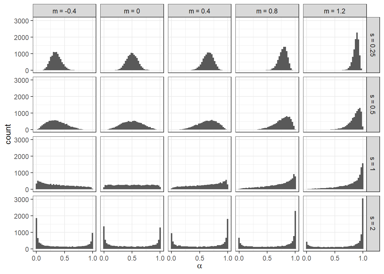
Figure 4.2: Histograms of 10,000 draws from the probit-normal distribution for various location ($m$) and scale ($s$) parameters.

For example Figure 4.2 shows a range of priors from the probit-normal family of distributions that we could use for our prior for the other-regarding preference parameter $\alpha$. In this figure, I especially want to draw your attention to the bottom row, which sets the prior scale parameter $s_\alpha$ to 2. If limited to these sixteen options, but without seeing Figure 4.2, one may be tempted to choose one of the priors with $s_\alpha=2$. This is because these priors have the largest variance. However inspection of the figure reveals that choosing one of these priors implies a starkly bi-model distribution for $\alpha$. To put this into context, these “uninformative” priors imply that it is very likely that $\alpha$ is close to one or zero, but very unlikely that it is anywhere in between. While $\alpha=1$ corresponds to self-regarding preferences, and so we may in fact like to have a fair chunk of prior probability mass near this value, the bunching at $\alpha=0$ should be particularly worrisome: this participant is completely selfless! In fact, we may even want to be worried about there being any appreciable mass in the $\alpha<0.5$ region, as this participant would place more weight on the other’s payoff than they do their own. My own assessment of this figure is that the $m=0.8$, $s=0.5$ panel covers the $0.5<\alpha<1$ region fairly well, and while not ruling it out, does not place too much mass in the $\alpha<0.5$ region.

While plotting alternative priors in something like Figure 4.2 can be helpful, another useful tool can be to write down a system of equations that pins down some properties that we would like the prior to have. Suppose for example that we think our prior should only place 1% probability mass on the $\alpha<0.5$ region. This could be because we believe that it is highly unlikey that people will care more about the other person’s payoff than their own. This condition tells us that:

\[ \begin{aligned} p(\alpha<0.5)&=0.01\\ p(\Phi^{-1}(\alpha)<\Phi^{-1}(0.5))&=0.01\\ p(X<0)&=0.01,\quad \text{where: }X=\Phi^{-1}(\alpha)\sim N(m_\alpha,s_\alpha^2)\\ \Phi\left(\frac{-m_\alpha}{s_\alpha}\right)&=0.01\\ -m_\alpha&=-2.33s_\alpha \end{aligned} \]

where $\Phi(x)$ is the standard normal cumulative density function, and $\Phi^{-1}(x)$ is its inverse.

As we have two parameters in the prior distribution to play with, we can choose one more property of the distribution. Therefore suppose that we want 20% of the probability mass to be in the $0.95<\alpha$ range, meaning that we expect there to be a large fraction of very self-regarding participants. This sets up the following equation:

\[ \begin{aligned} p(\alpha<0.95)&=0.8\\ p(X<1.64)&=0.8\\ \Phi\left(\frac{1.64-m_\alpha}{s_\alpha}\right)&=0.8\\ \frac{1.64-m_\alpha}{s_\alpha}&=0.842\\ m_\alpha&=1.64-0.842s_\alpha \end{aligned} \]

Adding the two conditions together gets us:

\[ \begin{aligned} 0&=1.64-3.17s_\alpha\\ s_\alpha& \approx 0.52 \end{aligned} \]

And then subtracting the first from the second:

\[ \begin{aligned} 2m_\alpha&=1.64-3.17\times 0.52+2.33\times0.52\\ m_\alpha\approx 1.2 \end{aligned} \]

which is not too far off the prior I selected by eyeballing Figure 4.2. Note that the parameter $m_\alpha$ pins down the prior median for $\alpha$, which is $\Phi(1.2)\approx0.88$. While an explicit expression for the mean of the probit-normal distribution does not exist, we can approximate it with Monte Carlo integration:

rnorm(1000,mean = 1.2,sd=0.52) |> pnorm() |> mean()

## [1] 0.85508

Of course, if we had some estimates of our parameters from previous studies, then these could also aid us in choosing a prior. For example in Bland (2023b), I calibrate a prior for risk-aversion using a distribution of estimates for a treatment reported in Holt and Laury (2002). Even better than this, the population-level estimates we get from hierarchical models have exactly the right interpretation we need to be priors for individual-level parameters. Therefore, if we have existing data that could speak to the parameters of a model we want to estimate, using these data to appropriately calibrate our priors could be very helpful.

4.3.2 Predictions and other derived quantities: The prior predictive check

A parameter like $\alpha$ can be relatively easy to interpret on its own: it represents the weight a participant places on their own payoff. However this is not always the case. For example, I find the logit choice precision parameter $\lambda$ difficult to interpret. For one thing, its units are inverse utility units, whatever they are. Furthermore, without a sense of the scale of payoffs in an experiment, it is difficult to know what a particular value of $\lambda$ implies for actual behavior. Fortunately, we can always transform a parameter, or group of parameters, into probabilistic predictions of behavior in our experiment (otherwise we would not be able to write down a likelihood), and so we can explore the implications of the more difficult-to-interpret parameters’ priors using these predictions. Additionally, we can also transform our parameters into other, economically meaningful quantities, that may be easier to interpret. For example in an experiment on decision-making under risk, the parameters in our structural model might permit us to compute a certainty equivalent, which is a translation of von-Neumann-Morgenstern utility units into currency. The latter I find much easier to interpret.

For the logit choice precision parameter $\lambda$, I like to think about its implications for choice probabilities. To see how to do this, note that for a given utility difference $\Delta>0$, the probability of choosing the action that yields the greatest utility is $(1+\exp(-\lambda\Delta))^{-1}$. Hence, if we have a sense of the scale of utility differences in our experiment, we can get a sense of the influence $\lambda$ has on choice probabilities. For Bruhin, Fehr, and Schunk (2019) for example, we can look at the unique values of the utility difference, evaluated at the prior median $\alpha$ of 0.88:

alpha<-0.88
Delta<-BFS2019 |>
  mutate(DU = (alpha*self_x+(1-alpha)*other_x-alpha*self_y-(1-alpha)*other_y) |> abs()) |>
  dplyr::select(DU) |>  unique() |> unlist() |> as.vector()

Delta

##  [1]  80.0 214.4 334.4 247.2 148.8 214.4 116.0  80.8 212.8 199.2 247.2 212.8
## [13]  45.6  80.0  10.4 184.0 116.0 148.8  45.6  10.4 302.4 334.4  80.8 302.4
## [25] 199.2  80.8  80.0 247.2 184.0  10.4 148.8 199.2  45.6 116.0

d<-expand.grid(
  Delta = Delta,
  lambda = 10^(seq(-5,1,length=1000))
  ) |>
  mutate(
    Pr = 1/(1+exp(-lambda*Delta))
  )

(
  ggplot(d,aes(x=lambda,y=Pr,group=Delta))
  +geom_path()
  +theme_bw()
  +scale_x_continuous(trans="log10")
  +xlab(expression(lambda))+ylab("Probability of choosing action with higher utility")
)

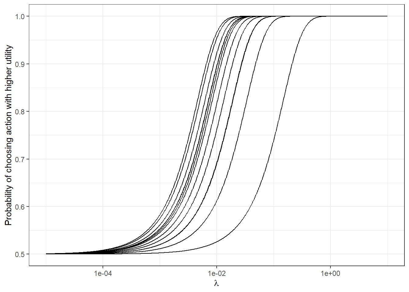
$The implications of choice precision $\lambda$ on choice probabilities.$

Figure 4.3: The implications of choice precision $\lambda$ on choice probabilities.

We can then plot the logit choice rule as a function of $\lambda$ to see how choice probabilities could change with $\lambda$. This is done in Figure 4.3. Here we can see that for $\lambda<10^{-4}$, all decisions are effectively coin flips: we might not want to assign too much prior probability in this region. Likewise for $\lambda>1$, decisions are effectively deterministic. Suppose then, that we decide to assign 99% of our prior probability to the region $10^{-4}<\lambda<1$, and use these endpoints as the 0.5th and 99.5th percentiles of the prior. This gives us a system of equations to solve for $m_\lambda$ and $s_\lambda$:

\[ \begin{aligned} -2.57s_\lambda&=\log(10^{-4})-m_\lambda\\ 2.57s_\lambda&=\log(1)-m_\lambda \end{aligned} \]

Adding them together yields:

\[ \begin{aligned} 2m_\lambda&=\log(10^{-4})+\log(1)\\ m_\lambda&\approx-4.61 \end{aligned} \] Subtracting the first from the second yields:

\[ \begin{aligned} 2\times2.57 s_\lambda &=\log(1)-\log(10^{-4})\\ s_\lambda&\approx 1.79 \end{aligned} \]

If we code it up the right way, we can also have our Stan model help us in choosing a prior. This is because we can always turn off the likelihood contribution with an appropriately-placed if statement. This is done using the UseData variable in the Stan model above. For the calibrated priors for $\alpha$ and $\lambda$, I simulate the prior predictive distribution of choices. I then summarize these distributions in Figure 4.4. This provides a useful “sanity check” to test whether or not our priors are implying anything weird about choices in the experiment.

PriorCheck<-"Code/Priors/priorCheck.rds" |>
  readRDS() |>
  data.frame() |>
  arrange(mean)

PriorCheck<-PriorCheck[rownames(PriorCheck)!="lp__",]
  
PriorCheck<-PriorCheck |>
  mutate(cumul = (1:n())/n())

(
  ggplot(PriorCheck,aes(x=mean,y=cumul))
  +geom_point()
  +geom_errorbar(aes(xmin = X25.,xmax = X75.))
  +geom_errorbar(aes(xmin = X2.5.,xmax = X97.5.),alpha=0.2)
  +theme_bw()
  +ylab("Cumulative density of prior mean")
  +xlab("Choice probability")
)

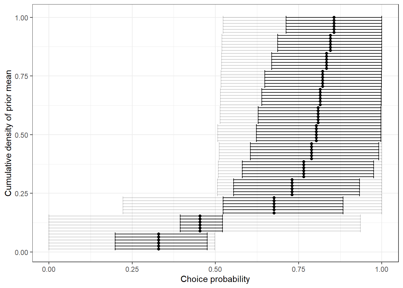
Prior distribution of choice probabilities. Dots show prior means. Heavy error bars show a 50% Bayesian credible region, and light error bars show a 95% Bayesian credible region.

Figure 4.4: Prior distribution of choice probabilities. Dots show prior means. Heavy error bars show a 50% Bayesian credible region, and light error bars show a 95% Bayesian credible region.

4.4 Assessing the sampling performance of a prior

Another way to investigate the implications of a prior is to explore the sampling properties of our estimator. As we have a probabilistic model, this can be done through simulation. That is, since we have a likelihood, we can draw simulated data from $y\mid \theta$, the distribution of $y$ given a specific realization of parameters $\theta$. Furthermore, since we also have a prior, we can simulate data that are consistent with our prior belief about these $\theta$s. In particular, the following simulation process:

Draw parameters $\tilde\theta$ from the prior
Draw data $y\mid\tilde\theta$ using the likelihood
Simulate the posterior $\theta\mid y$ using the simulated data.

produces data (in step 2) and estimates (in step 3) that are consistent with our prior. This information will let us do two important diagnostics of our estimation process. Firstly, we can ask if the model recovers its parameters well. That is, are our estimates $\hat\theta$ in some sense “close” to their true value $\theta$? Secondly, we can check whether our model is showing any pathologies by comparing the posterior distributions to the prior distribution. That is if all is working correctly, then draws from the prior in step 1 should have the same distribution as the posterior draws from step 3.

I demonstrate how this simulation is done in the R code at the end of this chapter. Basically, we first use Stan to get us some parameter draws from the prior distribution, and one simulated dataset consistent with each of these prior draws. I do this by running my Stan program with the UseData variable set to zero. Then for each of these simulated datasets, we fit the model and store the posterior draws.¹³

4.4.1 Does our model recover its parameters well?

A useful diagnostic for our model is to ask whether it estimates our parameters or quantities of interest well. Using the simulation described above, we can compare our posterior means to the prior draws that generated them. I show an example of this in Figure 4.5. Each dot represents a simulated dataset, with the horizontal coordinate equal to the (true) prior draw of $\alpha$ that generated the dataset, and the vertical coordinate equal to the posterior mean of $\alpha$. Ideally, all of these points would fall on the $45^\circ$ line (red dashed line), however we can expect the posterior mean to be pulled at least a little bit toward the prior mean, hence the smoothed fit (blue curve) crossing the $45^\circ$ line. Of course, this plot is just as much a function of your chosen prior as it is of your likelihood and experiment design. If this plot is not to your liking, then re-designing your experiment at this stage could go a long way.¹⁴

ParamRecovery<-readRDS("Code/Priors/SimSummary.rds") |>
  group_by(SimStep,alpha_true,lambda_true,alpha_MLE,lambda_MLE) |>
  summarize(alpha = mean(alpha),lambda = mean(lambda))

(
  ggplot(ParamRecovery,aes(x=alpha_true,y=alpha))
  +geom_point(size=1,alpha=0.5)
  +theme_bw()
  +geom_abline(intercept=0,slope=1,linetype="dashed",color="red")
  +geom_smooth(formula="y~x",method="loess")
  +geom_vline(xintercept=pnorm(1.2),color="red")
  +xlab("True value")
  +ylab("Posterior mean")
  +ylim(c(0,1))
)

$Parameter recovery plot for $\alpha$$

Figure 4.5: Parameter recovery plot for $\alpha$

In fairness to the Bayesian model, I also did the same exercise using the maximum likelihood estimator. The calibration plot can be seen below in Figure 4.6. Here there is clearly much more variance in the estimates, with a fair number of instances where the estimate falls at one of the endpoints of the parameter space.

(
  ggplot(ParamRecovery,aes(x=alpha_true,y=alpha_MLE))
  +geom_point(size=1,alpha=0.5)
  +theme_bw()
  +geom_abline(intercept=0,slope=1,linetype="dashed",color="red")
  +geom_smooth(formula="y~x",method="loess")
  +geom_vline(xintercept=pnorm(1.2),color="red")
  +xlab("True value")
  +ylab("Posterior mean")
  +ylim(c(0,1))
)

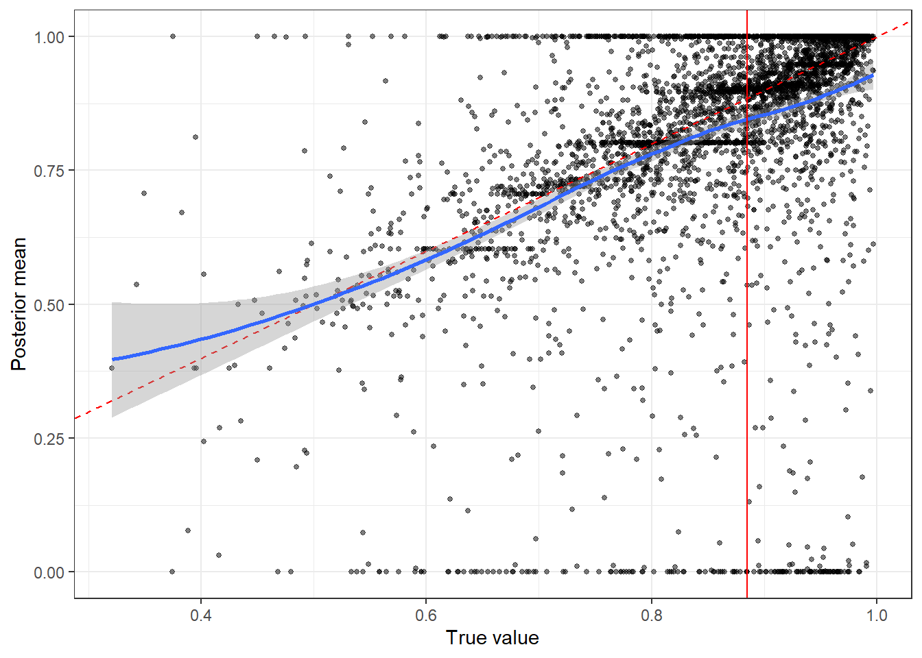
$Parameter recovery plot for $\alpha$ using maximum likelihood estimation$

Figure 4.6: Parameter recovery plot for $\alpha$ using maximum likelihood estimation

4.4.2 Do we see any pathologies in the estimation process?

Another sanity check for our prior and model that we can do with the above simulation process is to compare the draws from the prior to the draws from the posteriors. This is because the average posterior distribution should be the prior distribution (see Betancourt (2020) Section 1.2). We can do this by computing the rank of each prior draw within its corresponding posterior distribution (that we estimated using the dataset simulated from that prior draw). Then, if we plot the histogram of these ranks, we should get something close to a uniform distribution, which is what we get in Figure 4.7. I show these histograms alongside a 95% range for the binomial distribution (using the normal approximation) in order to give you a perspective for what normal statistical variation should look like.¹⁵ It is common for computational problems to manifest themselves in easy-to recognize ways in these plots (Betancourt 2020).

Rank<-readRDS("Code/Priors/SimSummary.rds") |>
  group_by(SimStep) |>
  summarize(
    alpha = sum(mean(alpha_true)<alpha),
    lambda = sum(mean(lambda_true)<lambda),
  ) |>
  pivot_longer(cols = c(alpha,lambda),names_to="parameter",values_to = "rank")


SimSize<-Rank$SimStep |> max()
nbins<-20

(
  ggplot(Rank,aes(x=rank))
  +geom_histogram(bins=nbins)
  +facet_wrap(~parameter)
  +theme_bw()
  +geom_hline(yintercept = SimSize/nbins,color="red")
  +geom_hline(yintercept = SimSize/nbins+1.96*sqrt(SimSize*(1/nbins)*(1-1/nbins)),color="red",linetype="dashed")
  +geom_hline(yintercept = SimSize/nbins-1.96*sqrt(SimSize*(1/nbins)*(1-1/nbins)),color="red",linetype="dashed")
)

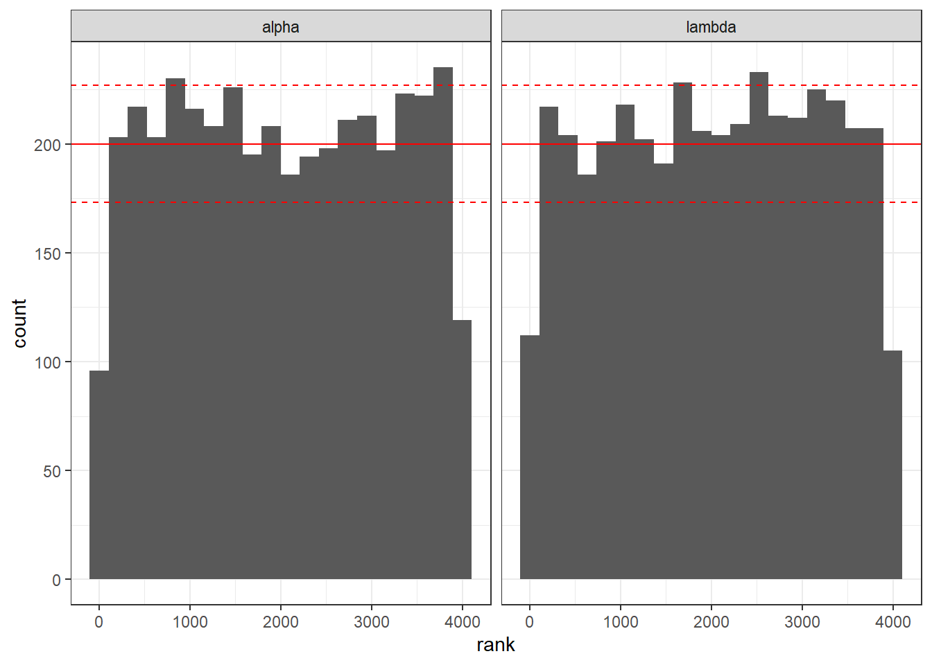
Figure 4.7: Histograms of ranks of prior draws within their corresponding posterior simulations.

Alternatively, we could visualize these ranks as an empirical cumulative density function, as I have done in Figure 4.8. Here, we are hoping that the plot will be of a straight line.

(
  ggplot(Rank,aes(x=rank))
  +stat_ecdf()
  +facet_wrap(~parameter)
  +theme_bw()
  +geom_abline(intercept=0,slope = 1/SimSize,color="red",linetype="dashed")
)

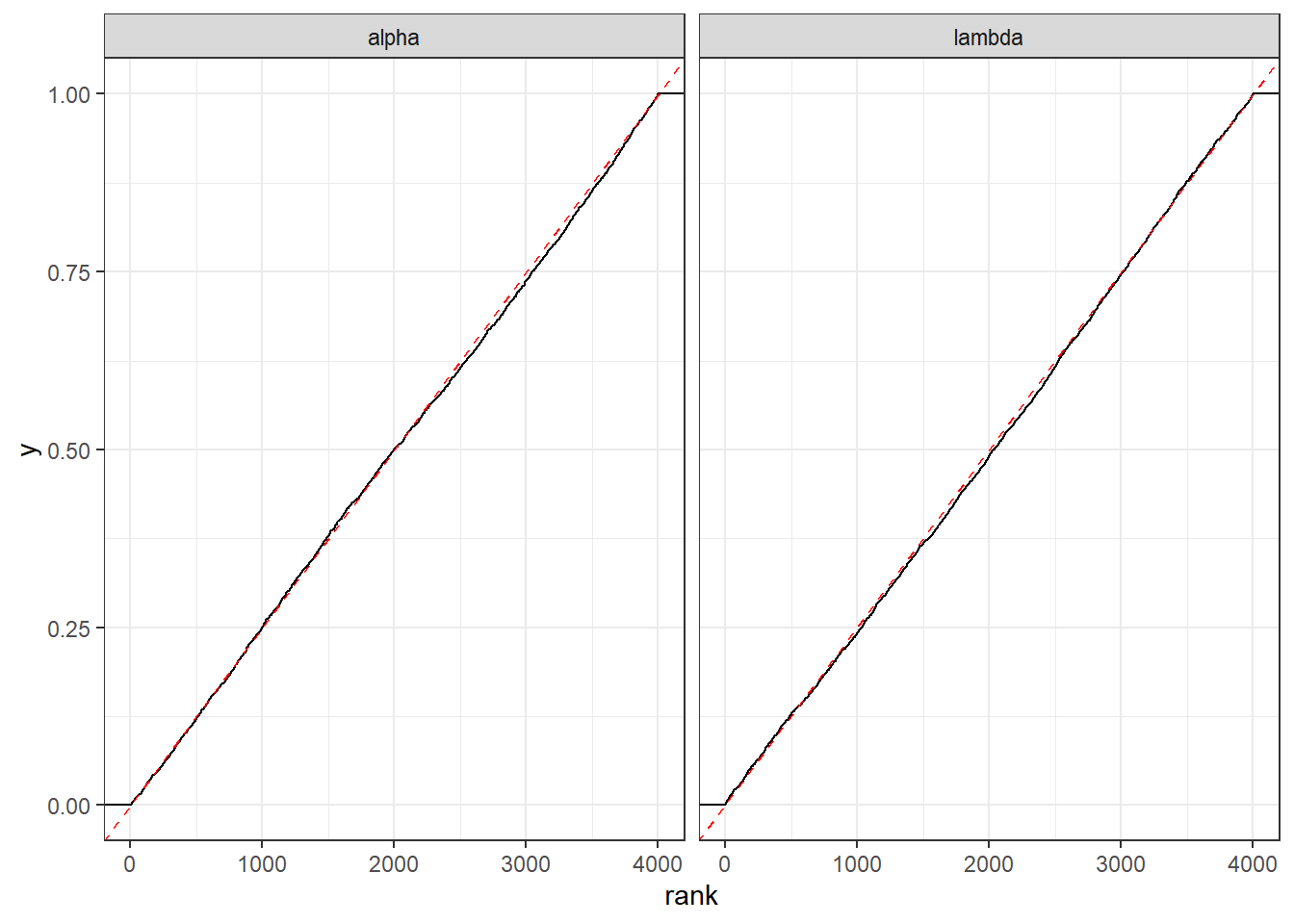
Empirical cumulative density function of ranks of prior draws within their corresponding posterior simulations. Dashed red line shows the ideal case of a uniform distribution.

Figure 4.8: Empirical cumulative density function of ranks of prior draws within their corresponding posterior simulations. Dashed red line shows the ideal case of a uniform distribution.

4.5 R code used for this chapter

library(tidyverse)
library(rstan)
  # These models estimate a lot faster without parallelization
  # This is because the initialization of the cores takes much
  # longer than the estimation itself
  options(mc.cores = 1)
  #options(mc.cores = parallel::detectCores())
  rstan_options(auto_write = TRUE)
  rstan_options(threads_per_chain = 1)
  
model<-stan_model("Code/Priors/BFS2019priors.stan")

# Load the data

d1<-(read.csv("Data/BFS2019_choices_exp1.csv")
     |> mutate(experiment=1)
)
d2<-(read.csv("Data/BFS2019_choices_exp2.csv")
     |> mutate(experiment=2)    
)
D<-(rbind(d1,d2)
    # Just use the dictator game data
    |> filter(dg==1)  
    |> mutate(
      self_alloc = ifelse(choice_x==1,self_x,self_y),
      other_alloc = ifelse(choice_x==1,other_x,other_y)
    )
)

# Data from just one participant
BFS2019<-D |> filter(sid==102010050706)

# Checking that it works
dStan<-list(
  n = dim(BFS2019)[1],
  y = BFS2019$choice_x,
  self_x = BFS2019$self_x,
  self_y = BFS2019$self_y,
  other_x = BFS2019$other_x,
  other_y = BFS2019$other_y,
  
  prior_lambda = c(-4.61,1.79),
  prior_alpha = c(1.2,0.52),
  UseData = 1,
  UsePrior = 1
)

Fit<-sampling(model,data=dStan,seed=42)  

## Simulating the prior distribution of choices

dStan$UseData<- 0
Fit<-sampling(model,data=dStan,seed=42,
              pars = "probX",include=TRUE)  
summary(Fit)$summary |> saveRDS("Code/Priors/priorCheck.rds")

## Simulating some data from the prior, then estimating the models
# using those data

SimData<-sampling(model,data=dStan,seed=42,
              pars = "probX",include=FALSE)

SIMDATA<-extract(SimData)$simX
  SIMDATA |> saveRDS("Code/Priors/SimData.rds")
alpha<-extract(SimData)$alpha
lambda<-extract(SimData)$lambda

dStan$UseData<-1

SimSummary<-tibble()

for (ss in 1:dim(SIMDATA)[1]) {
  print(paste("Sim step",ss,"of",dim(SIMDATA)[1]))
  
  # Estimate the model
  dStan$y<-SIMDATA[ss,] |> as.vector()
  Fit<-sampling(model,data=dStan,seed=42,
                pars = c("alpha","lambda"),include=TRUE)
  
  # Also check to see what the MLE looks like
  dStanMLE<-dStan
  dStanMLE$UsePrior<-0
  
  MLE<-optimizing(model,data=dStanMLE,seed=42)
  
  SimSummary<-rbind(
    SimSummary,
    tibble(
    SimStep = ss,
    alpha_true = alpha[ss],
    lambda_true = lambda[ss],
    alpha = extract(Fit)$alpha,
    lambda = extract(Fit)$lambda,
    alpha_MLE = MLE$par["alpha"],
    lambda_MLE = MLE$par["lambda"]
    )
  )
}

SimSummary |> saveRDS("Code/Priors/SimSummary.rds")

References

Betancourt, Michael. 2020. “Towards a Principled Bayesian Workflow.” https://betanalpha.github.io/assets/case_studies/principled_bayesian_workflow.html.

———. 2023b. “Bayesian Model Selection and Prior Calibration for Models of Behavior in Economic Experiments.” https://papers.ssrn.com/sol3/papers.cfm?abstract_id=4334267.

Bruhin, Adrian, Ernst Fehr, and Daniel Schunk. 2019. “The Many Faces of Human Sociality: Uncovering the Distribution and Stability of Social Preferences.” Journal of the European Economic Association 17 (4): 1025–69.

Holt, Charles A, and Susan K Laury. 2002. “Risk Aversion and Incentive Effects.” American Economic Review 92 (5): 1644–55.

Probably the biggest difference other than the prior is the differing approach to dealing with unobservable heterogeneity, which we will get to in the hierarchical models chapter.↩︎
If you have read other chapters of this book, you can see that I am a big fan of using this technique, at least as a starting point.↩︎
Coupled with the logit probabilistic choice rule, this means we will have two parameters total. This makes plotting parameter values much easier compared to a 3+ parameter model.↩︎
The process is simple, but took a while (a couple of hours on my laptop). If you’re playing at home, now would be a good time to slay a few lynels.↩︎
For this experiment in particular, which was not designed to estimate this utility function, I suspect that including more decisions where the allocations are connected by a line segment with a negative slope would improve this plot dramatically. This is because the indifference curves of the utility function that we are using will be downward-sloping, parallel, straight lines. Bruhin, Fehr, and Schunk (2019) designed this experiment with inequality-aversion in mind, rather than the efficiency-loving model that I use here. ↩︎
Betancourt (2020) also does this, it is not my original idea.↩︎