1 Introduction

1.1 What does your theory say about your data?

If you are reading this book, I can assume that you are interested in estimating an economic model of how people behave in a particular environment. But what does it mean to “estimate” an economic model? When we talk of estimating models, we usually mean econometric models. For example we might estimate the coefficients $\beta$ in a linear regression model:

\[ Y_i=\beta_0+\beta_1X_i+\epsilon_i \]

From my perspective, this equation is a model for how (say) treatment conditions in an experiment $X_i$ influence choices made by the experiment’s participants $Y_i$. The model assumes a linear relationship between $X$ and $Y$. The parameters of this model $(\beta_0,\beta_1)^\top$ describe the specific linear relationship that exists in the data, and our goal in linear regression is to estimate (and hopefully interpret) these parameters. While there are some special cases in which our theory will tell us that there should be a linear relationship between $X$ and $Y$,¹ this framework is woefully limiting relative to the rich set of economic models we might want to take to our data. Instead, we need a framework for translating our theoretical ideas about how our participants might behave into probabilistic predictions about what the data these participants generate will look like.

To fix ideas, suppose that in our experiment, we elicit participants’ risk preferences using an investment task:

You are endowed with 100 tokens, and can invest any amount of these tokens in a lottery. You have a chance of $1/2$ (50%) to win [$X$] times the tokens you bet on the lottery, and a $1/2$ (50%) chance that these tokens are lost. (adapted from Bland (2019))

We have an economic model, expected utility maximization, that makes predictions in this environment. Specifically, let $y^*$ be the number of tokens that a participant chooses to invest, then they will choose $y^*$ such that:

\[ y^*=\arg\max_{y\in[0,100]}\left\{0.5 u(100-y)+0.5 u(100-y + Xy)\right\} \]

where $u(x)$ is the participant’s utility function over certain amounts of money. We further make the simplifying assumption that this utility function takes on the constant relative risk-aversion functional form:

\[ u(x)=\frac{x^{1-r}}{1-r} \]

From here, we can solve the maximization problem using the first-order condition (please bear with me, I like to show my working):

\[ \begin{aligned} \max_{y\in[0,100]}&\left\{0.5 \frac{(100-y)^{1-r}}{1-r}+0.5 \frac{(100-y + Xy)^{1-r}}{1-r}\right\}\\ 0&=-0.5(100-y^*)^{-r}+0.5(X-1)(100-y^*+Xy^*)^{-r}\\ (100-y^*)^{-r}&=(X-1)(100+(X-1)y^*)^{-r}\\ y^*&=\frac{100(1-(X-1)^{-1/r})}{(X-1)^{1-1/r}+1} \end{aligned} \]

Which makes predictions that look like this:

library(tidyverse)
dplt1<-(
  expand.grid(X=seq(2.01,6,length=100),r = c(0.2,0.4,0.6,0.8))
  %>% mutate(y=100*(1-(X-1)^(-1/r))/((X-1)^(1-1/r)+1),
             r = paste("r =",r)
             )
)

(
  ggplot(dplt1,aes(x=X,y=y,color=r))
  +geom_path()
  +xlab("X")+ylab("y (optimal choice)")
  +theme_bw()
  
)

$Predictions from a model of expected utility maximization. $r$ is the parameter in the CRRA utility function $u(x)=\frac{x^{1-r}}{1-r}$$

Figure 1.1: Predictions from a model of expected utility maximization. $r$ is the parameter in the CRRA utility function $u(x)=\frac{x^{1-r}}{1-r}$

How would you go about estimating $r$? The relationship certainly isn’t linear. The solution I will teach you in this book is to modify the model so that it makes probabilistic predictions, rather than the deterministic predictions made in the figure above. Firstly, this is useful because it means that we can write down a likelihood function. This permits us to estimate our model using the Bayesian techniques described in this book, or maximum likelihood techniques if that is your thing. If done right, this is also a behaviorally plausible extension of the model with deterministic choice: like ourselves, our experiments’ participants are not infallible, and so will choose something different to our model’s point prediction. Furthermore, and perhaps more importantly, it is heroic to assume that the deterministic model of choice we wrote down above is exactly what our participants are doing, so having a component of choice that is not explicitly accounted for in the model is probably a good idea.

For this example, a probabilistic extension to the model could involve adding an error term to the end of our prediction:

\[ y=\frac{100(1-(X-1)^{-1/r})}{(X-1)^{1-1/r}+1}+\epsilon,\quad \epsilon\sim N(0,\sigma^2) \]

Or perhaps specifying a logistic choice rule, where choices that yield greater utility are more likely to be made than choices that yield less utility:

\[ \Pr(y=k)=\frac{\exp\left(\lambda\left(0.5\frac{(100-k)^{1-r}}{1-r}+0.5\frac{(100+(X-1)k)^{1-r}}{1-r}\right)\right)}{\sum_{j=1}^{100}\exp\left(\lambda\left(0.5\frac{(100-j)^{1-r}}{1-r}+0.5\frac{(100+(X-1)j)^{1-r}}{1-r}\right)\right)} \]

For example, the predictions using the logistic choice rule with $\lambda=10$ are now probability distributions:

r<-0.4
lambda<-10
dplt<-(
  expand.grid(X = c(2.25,2.75,3.5,5.5),y=seq(0,100,length=101),r=c(0.2,0.4,0.6,0.8))
  %>% mutate(EU = 0.5*(100-y)^(1-r)/(1-r)+0.5*(100+y*(X-1))^(1-r)/(1-r))
  %>% group_by(X,r)
  %>% mutate(pr = exp(lambda*(EU-max(EU)))/sum(exp(lambda*(EU-max(EU)))))
  %>% mutate(X=paste("X =",X),
             r=paste("r =",r))
)

(
  ggplot(dplt,aes(x=y,y=pr))
  +geom_path()
  +facet_grid(r~X,scales="free")
  +theme_bw()
  +xlab("Tokens invested")
  +ylab("probability")
)

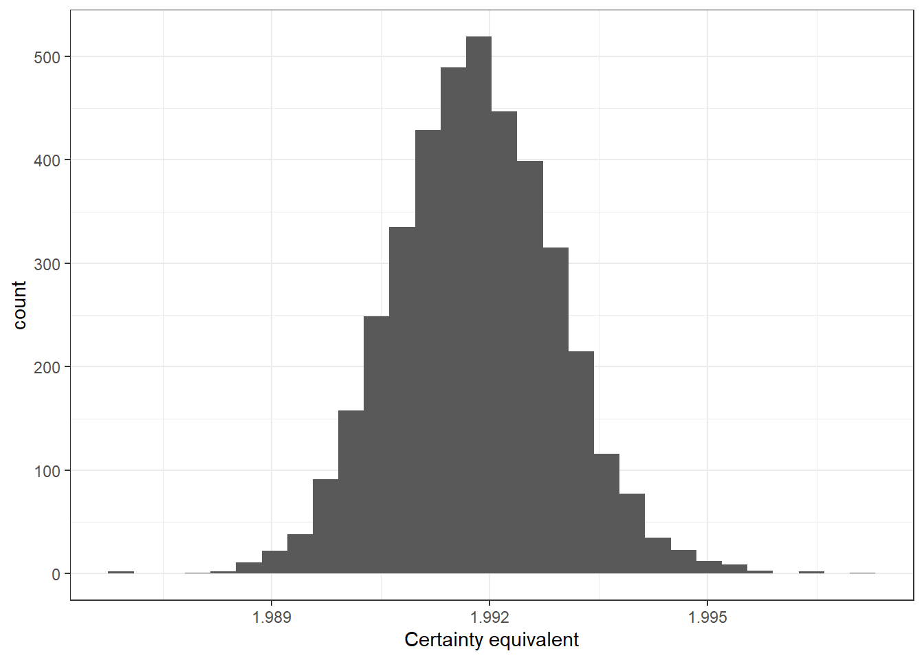
Figure 1.2: Probabilistic predictions for the investment task using a logistic choice rule

An added benefit of having a probabilistic model of behavior, even if we do not intend to estimate it, is that we can simulate data for our experiment. This can be useful both for experiment design, and for evaluating the sampling properties of our estimators. For example, suppose we wanted to see what the choices of a participant in this experiment would look like if they had $r=0.4$ and $\lambda=10$. The process for simulating data is very similar to the process for constructing the probability distribution:

r<-0.4
lambda<-10
set.seed(42)
probDist<-(
  expand.grid(y=seq(0,100,length=101),
              X = seq(2.5,6,length=30)
              )
  %>% mutate(EU = 0.5*(100-y)^(1-r)/(1-r)+0.5*(100+y*(X-1))^(1-r)/(1-r))
  %>% group_by(X)
  %>% mutate(pr = exp(lambda*(EU-max(EU)))/sum(exp(lambda*(EU-max(EU)))))
)

data<-tibble()

for (xx in (probDist$X %>% unique())) {
  d<-probDist %>% filter(X==xx)
  dataY<-sample(d$y,1,replace=TRUE,prob=d$pr)
  data<-rbind(data,
              tibble(y=dataY,X=xx))
}

(
  ggplot()
  +geom_point(data=data,aes(x=X,y=y))
  +geom_path(data=dplt1,aes(x=X,y=y,color=r))
  +xlab("X")+ylab("y (choice)")
  +theme_bw()
)

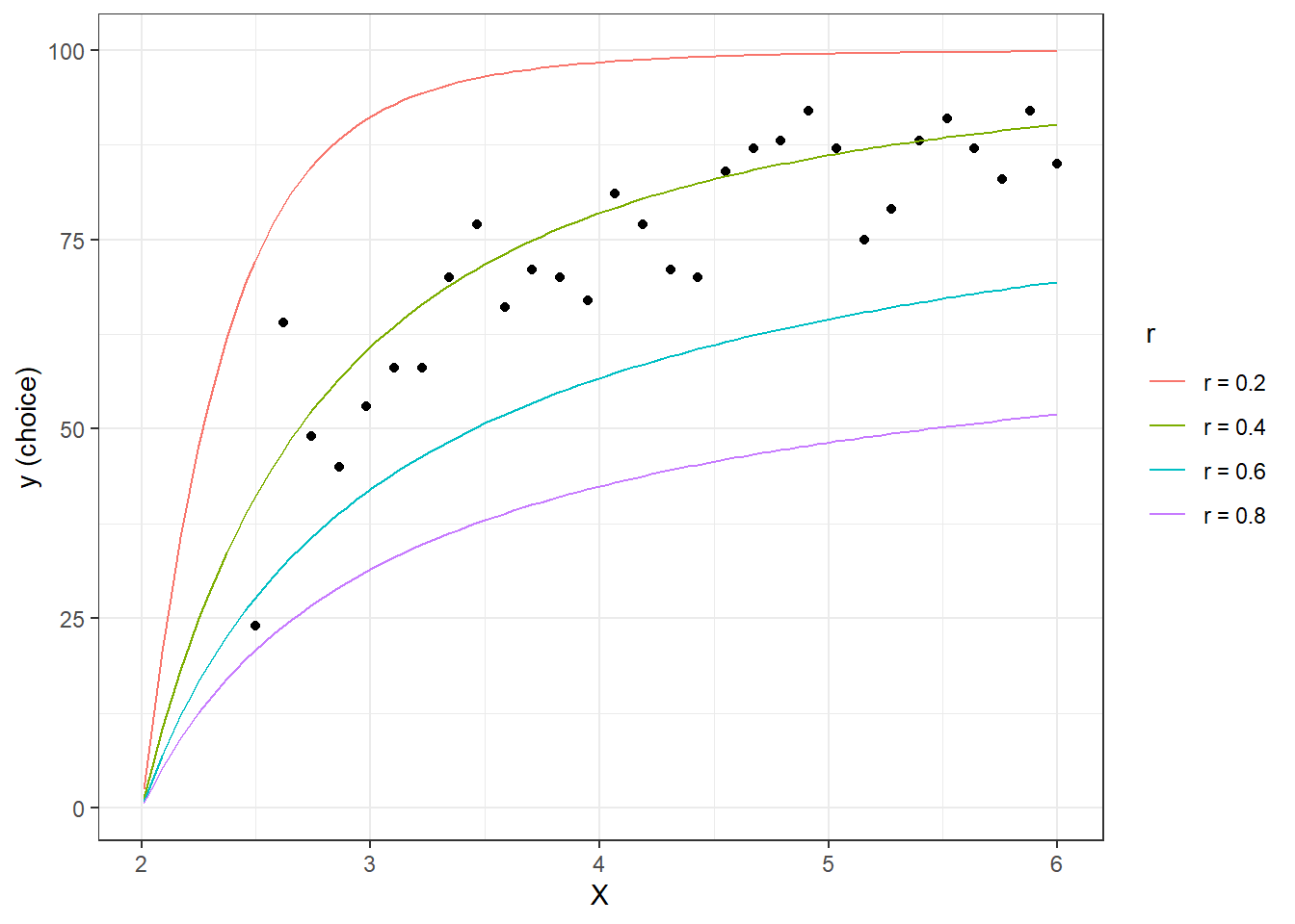
Figure 1.3: Some simulated data

This kind of simulation exercise is immensely useful. Graphically, we can see that if we want to estimate $r$ using this model and experiment, we will be trying to find the curve in Figure 1.3 (or maybe one in between) that best matches the data. Our probabilistic model will do all of the work defining what “best” is in this case. From Figure 1.3, we can see that our model will likely do a good job at distinguishing between $r=0.2$, $r=0.4$, and $r=0.6$, but might have trouble if we want to resolve the uncertainty about $r$ to a finer resolution. Additionally, now that we have a simulated dataset with known parameters, we can see how well our model estimates these parameters (I do this in the next section). Finally, these predictions help us to understand the implications of the choice precision parameter $\lambda$ (e.g. how dispersed are data around their point predictions?), and identify treatment conditions ($X$) that are going to be more (large $X$) or less (small $X$) informative about $r$.

1.2 What do your data say about your theory?

From here, it is not too much of a leap to code the model in Stan. True, we need to have a good think about what are appropriate priors, and so on, but hopefully you can see that once we have a probabilistic model written down, we can code it up in a similar way to how we derived it. Specifically, note how we specified the expected utility variable EU, then calculated the logistic choice probabilities (softmax).

// Introduction_InvestmentTask.stan

/*
In the data block, we tell Stan how to read in the data we will be passing
it from R.
*/
data {
  int<lower=0> n; // number of observations
  int<lower=0> ny; // size of the choice set
  int y[n];   // choices made by participant
  vector[n] X;   // multiplier for investment
  vector[ny] ygrid; // possible values of y (i.e. the choice set)
  real prior_r[2]; // prior mean and sd for r
  real prior_lambda[2]; // prior mean and sd for log(lambda)
}

/*
In the prarameters block, we tell Stan what the model's parameters are, 
and any restrictions we need to place on them. Here we need to restrict 
lambda to be positive
*/

parameters {
   real r; // parameter in CRRA utility function x^(1-r)/(1-r)
   real<lower=0> lambda; // logit choice precision
}


/*
In the model block, we tell Stan how the data and priors contribute to the 
posterior density
*/
model {
  
  /*
  In this loop, I go through each observation in the data, calculate the 
  expected utility of each possible choice in the choice set, then use this to
  compute the implied probability distribution over actions for that observation.
  I then take the (log) probability of the action that was actually taken and 
  add it to the likelihood
  */
  for (ii in 1:n) {
    vector[ny] EU; // expected utility of choosing each action
    vector[ny] lpr;// (log) probability of choosing each action
    EU = 0.5*pow(100-ygrid,1.0-r)/(1.0-r)+0.5*pow(100+ygrid*(X[ii]-1),1.0-r)/(1.0-r);
    
    lpr = log_softmax(lambda*EU);
    
    /*
    increment the log-likelihood
    Stan's "target" is in log probability units.
    */
    target+=lpr[y[ii]];
  }
  
  // specify the priors for the parameters
  r ~ normal(prior_r[1],prior_r[2]);
  lambda ~ lognormal(prior_lambda[1],prior_lambda[2]);
}

Finally, we go back to R, or any other programming language that will run Stan, and estimate the model. Here I am binning choices into increments of ten to make the computation faster.

library(rstan)
rstan_options(auto_write = TRUE)
options(mc.cores = parallel::detectCores()) # Use all the cores

# Get a list of data that Stan can understand.
# Note here that I am rounding the data to the nearest 10 tokens. 
# This will speed up the computation a lot. 
stanData<-list(y=round(data$y/10),
               X=data$X,
               n=data$y %>% length(),
               ygrid = (1:10)*10,ny=10,
               prior_r = c(0.5,0.25),
               prior_lambda = c(log(10),0.5))

# This if statement isn't needed, but is there so I don't have to run Stan 
# every time I compile this book. 
if (!file.exists("Outputs/Introduction/Introduction_InvestmentTask.rds")) {
  # Fit the model in Stan
  Fit<-stan("Code/Introduction/Introduction_InvestmentTask.stan",
            data=stanData,
            seed=42)
  # Save the fitted model so I can access it later without having to run 
  # Stan again
  saveRDS(Fit,file = "Outputs/Introduction/Introduction_InvestmentTask.rds")
}
# Read in the saved fitted model 
Fit<-readRDS("Outputs/Introduction/Introduction_InvestmentTask.rds")

# Display a summary of the estimates
summary(Fit)$summary %>% knitr::kable(caption="Summary of the estimated *Stan* model.")

Table 1.1: Summary of the estimated *Stan* model.
	mean	se_mean	sd	2.5%	25%	50%	75%	97.5%	n_eff	Rhat
r	0.4150626	0.0001717	0.0075883	0.4001603	0.4100248	0.4151369	0.4201586	0.429389	1953.892	1.0007558
lambda	7.3300355	0.0306710	1.3916342	4.7949716	6.3154328	7.2493079	8.2539359	10.132982	2058.705	0.9993396
lp__	-62.8776918	0.0257126	1.0161700	-65.6160771	-63.2451930	-62.5697220	-62.1778855	-61.900278	1561.850	0.9997605

And that’s it! We have taken a model all the way from deriving predictions, expanding it to make probabilistic predictions, and finally to estimating the parameters in the model.

1.3 What do your parameters say about other things?

Let’s say that again: we estimated the parameters in the model!. We have a model that says that parameter $r$ is important, and here is everything we learned from it in our (simulated) experiment:

(
  ggplot(tibble(r=extract(Fit)$r),aes(x=r))
  +geom_histogram()
  +theme_bw()
)

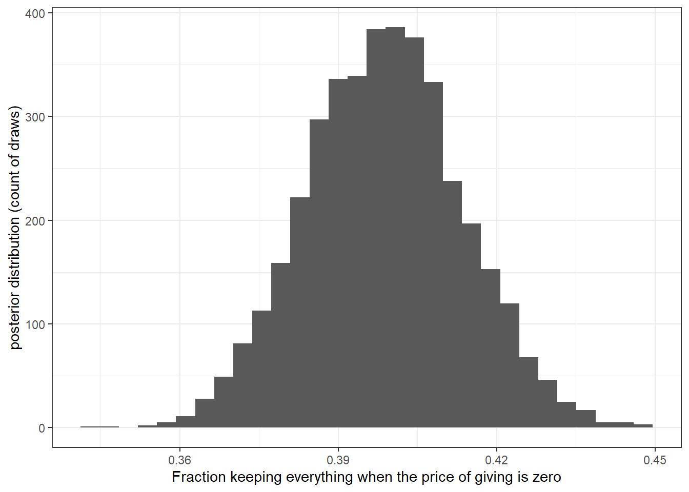
Figure 1.4: The posterior distribution of CRRA parameter $r$

But we do not have to stop here. In fact, the benefits of a structural model really start to be recognized here. Not only do we have estimates of our parameter, but because this is an economic model as well as an econometric model, we can also use it to make out-of-sample predictions. That is, we can take the model beyond the confines of the experiment we used to estimate it, and derive its implications in other environments.

For example, suppose that we were designing another experiment where this participant could choose between the following two lotteries:

$2.00 for sure
A 70% chance of $2.50, and a 30% chance of $1.00.

Our model tells us that they will prefer the risky Lottery 2 if and only if:

\[ 0.7\frac{2.5^{1-r}}{1-r}+0.3\frac{1^{1-r}}{1-r}\geq \frac{2^{1-r}}{1-r} \]

and since we have a posterior distribution of $r$, we can compute a posterior probability of this event being true:

r<-extract(Fit)$r
mean((0.7*2.5^(1-r)/(1-r)+0.3*1^(1-r)/(1-r)-2^(1-r)/(1-r))>=0)

## [1] 0

In other words, it is unlikely that this participant will prefer the risky lottery over the certain outcome.

Furthermore, one of the benefits of Bayesian estimation is that the posterior distribution of transformations of a model’s parameters can be accessed by simply transforming the model’s simulated posterior draws. That is, there are no pesky delta-method calculations to do if one wants to compute a nonlinear transformation of parameters. These show up in our models all the time. For example, we can use the model’s estimates to calculate the certainty equivalent of this risky lottery (i.e. the sure amount that makes the decision-maker indifferent to the risky lottery). Mathematically, we calculate:

\[ \begin{aligned} \frac{C^{1-r}}{1-r}&=0.7\frac{2.5^{1-r}}{1-r}+0.3\frac{1^{1-r}}{1-r}\\ C&=\left(0.7\times 2.5^{1-r}+0.3\times 1^{1-r}\right)^\frac{1}{1-r} \end{aligned} \] So our posterior distribution for $C$ is:

d<-(tibble(r=r)
  %>% mutate(C = (0.7*2.5^(1-r)+0.3*1^(1-r))^(1/(1-r)))   
)

(
  ggplot(data=d,aes(x=C))
  +geom_histogram()
  +theme_bw()
  +xlab("Certainty equivalent")
)

Figure 1.5: Posterior distribution of the certainty equivalent of the risky lottery

So we can be fairly sure that the certainty equivalent is about $2.

1.4 What does your expertise say about your parameters?

Of course, before we do any of this, as experts in our field we will actually have a reasonably good idea about what might happen in our experiments. True, we are running an experiment because we don’t know exactly what will happen. But our understanding of the environment, based on past observations, will surely guide us in designing the experiment, and Bayesian statistics permits this understanding to also guide us in analyzing our data.

We also use a probabilistic model to express our beliefs about our parameters. These are called priors. For example, in the model I estimated above, I stated that my belief for the risk-aversion parameter $r$ was:

\[ r\sim N(0.5,0.25^2) \] This can be seen in the R code where I specify:

prior_r = c(0.5,0.25)

in the data I pass to Stan, and then in the Stan program where I specify the prior:

r ~ normal(prior_r[1],prior_r[2])

Our priors are going to serve (at least) two purposes. Firstly, in the design stage of an experiment, they are going to help us assess which experimental conditions are the most useful to take to our participants. Coupled with a likelihood, they also permit us to simulate data of our experiment that is consistent with our prior beliefs about what our data will look like. This is immensely beneficial even if we do not take a Bayesian model to our data: by having simulated data representative of our prior, we can adjust our experimental conditions so as to best answer our research questions. Furthermore, it provides us with an opportunity to test whether our econometric analysis will be well suited to analyzing the data that comes from our experiment.

Secondly, in the estimation stage of your research workflow, your prior will help your model look for solutions to its data-fitting exercise that are economically plausible. Maximum likelihood estimates of models of choice under risk, for example, are known to be difficult to solve for some participants (see for example Harrison and Ng (2016)) because multiple maxima exist. A prior will re-weight the problem so that more emphasis is placed on parameter values that are ex-ante plausible (see for example Gao, Harrison, and Tchernis (2022), which uses the same dataset as Harrison and Ng (2016)).

However priors can be a double-edged sword: while we want our model to estimate parameters that are economically plausible, we do not want our models to be so overly-informed by a prior that they hardly learn from the data. There is a gentle balancing act in choosing a suitable prior for our models that on the one hand incorporates our understanding of the problem as experts in the field, and on the other hand are not so informative that we might as well not collect data. The solution is not to try to be “as uninformative as possible”, as this will open up another can of worms (e.g. Bland (2023b)). Instead, we should be methodical about asking not just what our priors say about their parameters, but also what our priors say about data, and quantities of interest that we might want to estimate and report. As such, much of this book will follow ideas laid out in Michael Betancourt’s Principled Bayesian Workflow (Betancourt 2020). I believe that this process strikes a practical balance between priors being (i) something set in stone because they are exactly our beliefs about things, and (ii) something we must worry about at all costs because they will bias our estimates if they are too informative. As such, we will put our priors through the wringer before we collect our data, and this will be to our benefit. This scrutiny will provide us with a deeper understanding of our models and the kind of data we might get from our experiments.

References

Betancourt, Michael. 2020. “Towards a Principled Bayesian Workflow.” https://betanalpha.github.io/assets/case_studies/principled_bayesian_workflow.html.

Bland, James R. 2019. “How Many Games Are We Playing? An Experimental Analysis of Choice Bracketing in Games.” Journal of Behavioral and Experimental Economics 80: 80–91. https://doi.org/10.1016/j.socec.2019.03.011.

———. 2023b. “Bayesian Model Selection and Prior Calibration for Models of Behavior in Economic Experiments.” https://papers.ssrn.com/sol3/papers.cfm?abstract_id=4334267.

Gao, Xiaoxue Sherry, Glenn W Harrison, and Rusty Tchernis. 2022. “Behavioral Welfare Economics and Risk Preferences: A Bayesian Approach.” Experimental Economics, 1–31. https://doi.org/10.1007/s10683-022-09751-0.

Harrison, Glenn W, and Jia Min Ng. 2016. “Evaluating the Expected Welfare Gain from Insurance.” Journal of Risk and Insurance 83 (1): 91–120. https://doi.org/10.1111/jori.12142.

For example, for a private-value first-price auction with independent uniform values, the equilibrium bidding function will take the form $\mathrm{bid}_i=\beta_0+\beta_1\mathrm{value}_i$.↩︎