12 Speeding up your Stan code
While Bayesian computation certainly isn’t for the impatient, there are some things you can do to make sure you are not waiting any longer than you have to for your results. I this chapter, I will show you some ways to write code that runs faster. In particular, we will learn about recognizing opportunities to pre-compute values, how to vectorize operations, and how to take advantage of Stan’s within-chain parallel processing capabilities. The first two of these will help on any machine that you might be using, whereas parallelization might help in specific instances where you have some idle cores that could be put to use.
12.1 Example dataset and model
In this chapter we will be estimating a two-parameter Expected Utility Theory (EUT) model for each of the 327 participants of Harrison and Swarthout (2023). In this experiment, each participant made 100 binary lottery choices. Each lottery pair can be described by three monetary prizes (which were common for both lotteries in the pair), and the probabilities of winning each prize. Let \(x_{t,k}\) be the \(k\)th prize in lottery pair \(t\), and \(q_{t,k}^L\) and \(q_{t,k}^R\) are the probabilities of winning prize \(k\) for the “Left” and “Right” lottery in pair \(t\). Assuming a constant relative risk-aversion specification, we can then write down the expected utility of the Left lottery in pair \(t\) as:
\[ Eu(x_t,q_{t}^L\mid r)=\sum_{k=1}^3q_{t,k}^L\frac{x_{t,k}^{1-r}}{1-r} \]
where \(r\in\mathbb R\) is the coefficient of relative risk-aversion.
I assume that the prizes are inclusive of the experiment’s \(\$10\) show-up fee, and the “endowment” for the lottery, which was used to frame some lottery pairs in the loss domain.
Using the contextual utility normalization (Wilcox 2011) and a logit choice rule with precision \(\lambda\) means that the probability of choosing the Left lottery in pair \(t\) is:
\[ p(y_t=\mathrm{Left}\mid r,\lambda)=\Lambda\left(\lambda\frac{\sum_{k=1}^3q_{t,k}^L\frac{x_{t,k}^{1-r}}{1-r}-\sum_{k=1}^3q_{t,k}^R\frac{x_{t,k}^{1-r}}{1-r}}{\frac{\overline x_{t}^{1-r}}{1-r}-\frac{\underline x_{t}^{1-r}}{1-r}}\right) \]
where \(\overline x_t\) and \(\underline x_t\) are the largest and smallest prizes in lottery pair \(t\), respectively.
I will use the priors suggested in James R. Bland (2025) for this model, which are:
\[ \begin{aligned} r&\sim N(0.27,0.36^2)\\ \log\lambda&\sim N(\log 30,0.5^2) \end{aligned} \]
The prior for \(r\) was calibrated to match estimates form Holt and Laury (2002), and the prior for \(\lambda\) was calibrated to achieve some plausible predictions based on the probabilistic choice rule.
12.2 A really slow way to estimate the model
I start out with a Stan program that looks like how I would code in Matlab in 2010: completely unaware of what makes code fast, but with a good understanding of how a for loop works! Here I compute the expected utility difference for each decision separately (in the for (ii in 1:N) loop), and for good measure also compute the sums in the expected utility formula using a for loop. There is nothing mathematically wrong with any of this, but as you will see below, we can speed things up considerably.
data {
  int<lower=0> N; // number of decisions

  int Left[N]; // logical =1 if left lottery was chosen

  matrix[N,3] prizes; // the 3 monetary prizes
  matrix[N,2] prizerange; // The minimum and maximum prize


  matrix[N,3] probL; // prob. distribution for Left lottery
  matrix[N,3] probR; // prob. distribution for Right lottery

  vector[2] prior_r; // normal prior on CRRA parameter
  vector[2] prior_lambda; // log-normal prior on logit choice precision
}

parameters {
  real r;
  real<lower=0> lambda;
}
model {

  // priors
  r ~ normal(prior_r[1],prior_r[2]);
  lambda ~ lognormal(prior_lambda[1],prior_lambda[2]);

  for (ii in 1:N) { // loop over lottery pairs

    real EUleft = 0.0;
    real EUright = 0.0;

    for (kk in 1:3) { // loop over lottery pairs
      // add each component of the sum individually
      EUleft += probL[ii,kk]*pow(prizes[ii,kk],1.0-r)/(1.0-r);
      EUright += probR[ii,kk]*pow(prizes[ii,kk],1.0-r)/(1.0-r);

    }
    // contextual utility normalization
    real normalizedUtility = (EUleft-EUright)/
                            (pow(prizerange[ii,2],1.0-r)/(1.0-r)-pow(prizerange[ii,1],1.0-r)/(1.0-r));

    target += bernoulli_logit_lpmf(Left[ii] | lambda*normalizedUtility);

  }

}
12.3 Pre-computing things
Probably the lowest-hanging fruit for speeding up your code is realizing when something can be calculated once, rather than every time Stan does an iteration. That is, if you can move something from the model or transformed parameters blocks into the transformed data block, then Stan will only have to do it once, instead of thousands of times.
For the EUT model presented above, note the following re-arrangement of the likelihood:
\[ \begin{aligned} p(y_t=\mathrm{Left}\mid r,\lambda)&=\Lambda\left(\lambda\frac{\sum_{k=1}^3q_{t,k}^L\frac{x_{t,k}^{1-r}}{1-r}-\sum_{k=1}^3q_{t,k}^R\frac{x_{t,k}^{1-r}}{1-r}}{\frac{\overline x_{t}^{1-r}}{1-r}-\frac{\underline x_{t}^{1-r}}{1-r}}\right)\\ &=\Lambda\left(\lambda\frac{\sum_{k=1}^3\frac{x_{t,k}^{1-r}}{1-r}\left(q^L_{t,k}-q^R_{t,k}\right)}{\frac{\overline x_{t}^{1-r}}{1-r}-\frac{\underline x_{t}^{1-r}}{1-r}}\right) \end{aligned} \]
That is, an EUT participant only cares about the difference in probabilities between two lotteries, and since these probabilities are not a function of the model’s parameters, we can compute their difference in the transformed data block. Here is my modification to the program that does this (the new data variable is called dprob):
data {
  int<lower=0> N; // number of decisions

  int Left[N]; // logical =1 if left lottery was chosen

  matrix[N,3] prizes; // the 3 monetary prizes
  matrix[N,2] prizerange; // The minimum and maximum prize


  matrix[N,3] probL; // prob. distribution for Left lottery
  matrix[N,3] probR; // prob. distribution for Right lottery

  vector[2] prior_r; // normal prior on CRRA parameter
  vector[2] prior_lambda; // log-normal prior on logit choice precision
}

transformed data {

  matrix[N,3] dprob = probL-probR;

}

parameters {
  real r;
  real<lower=0> lambda;
}
model {

  // priors
  r ~ normal(prior_r[1],prior_r[2]);
  lambda ~ lognormal(prior_lambda[1],prior_lambda[2]);

  for (ii in 1:N) { // loop over lottery pairs

    real DEU = 0.0;

    for (kk in 1:3) { // loop over lottery pairs
      // add each component of the sum individually
      DEU += dprob[ii,kk]*pow(prizes[ii,kk],1.0-r)/(1.0-r);

    }
    // contextual utility normalization
    real normalizedUtility = DEU/
                            (pow(prizerange[ii,2],1.0-r)/(1.0-r)-pow(prizerange[ii,1],1.0-r)/(1.0-r));

    target += bernoulli_logit_lpmf(Left[ii] | lambda*normalizedUtility);

  }

}
12.4 Vectorization
Now we will eliminate that nasty double for loop by replacing it with a matrix operation. This will speed things up because Stan is very fast at vector and matrix operations. Furthermore, a lot of Stan’s in-built functions are vectorized, and so we can even take advantage of this for non-linear functions (see below where I use pow(,)).
The trick here is to note that our expression for expected utility is a sum, and we can write a sum as an inner product. Since we have N of these sums, if we can write the terms of the sum as a matrix, we can compute all of the expected utilities as a matrix multiplication. First, note that all of the terms in the expression for \(Eu(x_t,p_t^L\mid r)\) can be written as:
\[ q^L \cdot \frac{x^{1-r}}{1-r} \]
where \(q^L\) is an \(N\times 3\) matrix representing the probabilities in the \(L\) lotteries, \(x\) is an \(N\times 3\) matrix representing the prizes in these lotteries, and \(\cdot\) indicates an element-wise matrix multiplication. Here we are raising \(x\) to the power of \(1-r\) element-wise. The result of this is an \(N\times 3\) matrix, where each row represents a lottery, and each column represents a prize. Now we need to add up the rows. This can be done by multiplying this matrix by a vector of ones:
\[ Eu(x,q^L\mid r)=\left(q^L \cdot \frac{x^{1-r}}{1-r}\right)\begin{pmatrix}1\\1\\1\end{pmatrix} \]
Carrying through our insight that we can pre-compute the difference in probabilities, we can further speed this up by just calculating the expected utility difference, which is all we need to compute the logit choice probability:
\[ Eu(x,q^L\mid r)-Eu(x,p^R\mid r)=\left((q^L-q^R) \cdot \frac{x^{1-r}}{1-r}\right)\begin{pmatrix}1\\1\\1\end{pmatrix} \]
Here is how I implement this in the Stan program:
Note the use of .* for the element-wise multiplication, and that the pow(.,.) function also does an element-wise operation (raising every element of prizes to the power of 1-r).
Finally, we can take advantage of the fact that bernoulli_logit_lpmf(.|.) is a reduction, so instead of writing a for loop to increment the likelihood:
for (ii in 1:N) {
target += bernoulli_logit_lpmf(Left[ii] | lambda * DEU[ii] ./
(pow(prizerange[ii,2],1.0-r)-pow(prizerange[ii,1],1.0-r))/(1.0-r)
);
}We can just input the whole vector DEU and integer array Left, and it will compute the sum of the individual log-likelihoods.
target += bernoulli_logit_lpmf(Left | lambda * DEU ./
(pow(prizerange[,2],1.0-r)-pow(prizerange[,1],1.0-r))/(1.0-r)
);Here is the whole Stan program:
data {
int<lower=0> N; // number of decisions
int Left[N]; // logical =1 if left lottery was chosen
matrix[N,3] prizes; // the 3 monetary prizes
matrix[N,2] prizerange; // The minimum and maximum prize
matrix[N,3] probL; // prob. distribution for Left lottery
matrix[N,3] probR; // prob. distribution for Right lottery
vector[2] prior_r; // normal prior on CRRA parameter
vector[2] prior_lambda; // log-normal prior on logit choice precision
}
transformed data {
matrix[N,3] dprob = probL-probR;
}
parameters {
real r;
real<lower=0> lambda;
}
model {
// priors
r ~ normal(prior_r[1],prior_r[2]);
lambda ~ lognormal(prior_lambda[1],prior_lambda[2]);
 vector[N] DEU = (
      dprob
      .*pow(prizes,1.0-r)/(1.0-r)
    )*rep_vector(1.0,3);
target += bernoulli_logit_lpmf(Left | lambda * DEU ./
        (pow(prizerange[,2],1.0-r)-pow(prizerange[,1],1.0-r))/(1.0-r)
    );
}12.5 Within-chain parallelization with reduce_sum()
If you have run any Stan program at all, you will probably be aware that it automatically gives you between-chain parallelization.53 That is, if your computer has more than one logical processor, and you use the recommended option options(mc.cores = parallel::detectCores()), RStan will run as many of the required chains as it can in parallel, which is four chains by default. This is great, because things should run about four times faster (if you have at least four logical processors).54 Stan also supports within-chain parallelization, which means that within a chain more than one computation can be done at a time, if your computer can support it.
In this section, I will show you how to use Stan’s reduce_sum() function (documentation here) to parallelize the computation of the log-likelihood. The trick here is realizing that since the log-likelihood is a sum, we can compute subsets of the sum in parallel (i.e. on separate processors), and then add up the results to get the grand total. That is, we can write the log-likelihood as the sum of the individual likelihoods of the 100 decisions made by the participant, then split these up into (say) four chunks of 25 decisions:
\[ \begin{aligned} \log p(y\mid \theta)&=\sum_{t=1}^{100} \log p(y_t\mid\theta)\\ &= \underbrace{\sum_{t=1}^{25} \log p(y_t\mid\theta)}_\text{to processor 1} +\underbrace{\sum_{t=26}^{50} \log p(y_t\mid\theta)}_\text{to processor 2} +\underbrace{\sum_{t=51}^{75} \log p(y_t\mid\theta)}_\text{to processor 3} +\underbrace{\sum_{t=76}^{100} \log p(y_t\mid\theta)}_\text{to processor 4} \end{aligned} \]
In principle if you have four processors, this should take a a bit more than a quarter of the time that the non-paralellized addition takes, but in practice there is substantial overhead in managing the parallelization. This means that you want to think carefully about which operations you parallelize, and how you chose tuning parameters for the parallelization (more on this later). In fact in the example below, I had to give Stan a more computationally intensive problem to showcase the benefits of within-chain parallelization: there really are no noticeable gains to be made if we just want to do the participant-specific estimation (at least on my machine).
In order to use reduce_sum(), you will need to write a user-defined function in the functions block that computes a chunk of the sum, returning a real number. In my code below, this function is called sum_likelihood(). reduce_sum() needs this function to have a specific signature, meaning that its arguments need to appear in a specific order, which is:
x_slice, the slice of the data that we will use to compute this chunk of the likelihoodstart, an integer identifying the first term of the data going into this chunkend, an integer identifying the last term of the data going into this chunk- Any remaining quantities we need to compute the sum
Here is the user-defined function I wrote to compute this chunk:
  real sum_likelihood(
    int[] Left,
    int start, int end,
    real lambda, real r,
    matrix dprob, matrix prizes, matrix prizerange
  ) {

    int n = end-start+1;

    vector[n] lambdaDEU = lambda*((dprob[start:end,] .*pow(prizes[start:end,],1.0-r))*rep_vector(1.0,3))
                                  ./
                                  (pow(prizerange[start:end,2],1.0-r)-pow(prizerange[start:end,1],1.0-r))
    ;

    return bernoulli_logit_lpmf(Left | lambdaDEU);

  }
That is, we could use this function without any within-chain parallelization to increment the likelihood as follows:
But since we do want to use within-chain paralleloization, we input this user-defined function into reduce_sum() like this:
Here grainsize is a (positive integer) tuning parameter for reduce_sum(), and refers to the maximum number of elements in a chunk of the sum to be sent off to a processor.
Stan’s documentation for choosing grainsize recommends choosing grainsize = 1 unless you spend some time investigating how this parameter affects performance. With this option selected, Stan will try to find a good way to split up the sum. For any other grainsize > 1, it follows your recommendation.
Here is the entire Stan program. I have coded it with an option doparallel, which allows for toggling whether or not within-chain parallelization is used. That way when I look for any improvements due to parallelization, I will be running everything from the same Stan program.
functions {
real sum_likelihood(
int[] Left,
int start, int end,
real lambda, real r,
matrix dprob, matrix prizes, matrix prizerange
) {
int n = end-start+1;
vector[n] lambdaDEU = lambda*((dprob[start:end,] .*pow(prizes[start:end,],1.0-r))*rep_vector(1.0,3))
./
(pow(prizerange[start:end,2],1.0-r)-pow(prizerange[start:end,1],1.0-r))
;
return bernoulli_logit_lpmf(Left | lambdaDEU);
}
}
data {
int<lower=0> N; // number of decisions
int Left[N]; // logical =1 if left lottery was chosen
matrix[N,3] prizes; // the 3 monetary prizes
matrix[N,2] prizerange; // The minimum and maximum prize
matrix[N,3] probL; // prob. distribution for Left lottery
matrix[N,3] probR; // prob. distribution for Right lottery
vector[2] prior_r; // normal prior on CRRA parameter
vector[2] prior_lambda; // log-normal prior on logit choice precision
int grainsize;
int doparallel; // if ==1 then do within-chain parallelization
}
transformed data {
matrix[N,3] dprob = probL-probR;
}
parameters {
real r;
real<lower=0> lambda;
}
model {
// priors
r ~ normal(prior_r[1],prior_r[2]);
lambda ~ lognormal(prior_lambda[1],prior_lambda[2]);
if (doparallel==1) {
target += reduce_sum(
sum_likelihood,
Left,
grainsize,
lambda, r,
dprob, prizes, prizerange
);
} else {
target += sum_likelihood(Left,
                         1,N,
                         lambda,r,
                         dprob,prizes,prizerange
                           );
}
}12.6 Evaluating the implementations
As explained in more detail below, there are not any gains to be made from parallelization of the participant-specific estimation. I therefore start with evaluating the the performance of the other models, then turn to evaluating parallelization from a slightly different angle.
12.6.1 Pre-computing and vectorization
Here I estimate the three un-parallelized models for each participant in Harrison and Swarthout (2023), running RStan’s default options except for:
chains = 1, i.e. running only one chain, andrefresh = 1000, which only displays progress every 1,000 iterations
The computation times are summarized in Figure 12.1, which shows the empirical cumulative distributions of these times. The vectorized model runs almost four times faster than the original “slow” model.
BenchmarkSummary<-"Code/SpeedyCode/BenchmarkSummarySeries.rds" |>
  readRDS()

d<-BenchmarkSummary |>
  group_by(id,model) |>
  summarize(
    time = mean(time)
  )

(
  ggplot(d ,aes(x=time,color=model))
  +stat_ecdf()
  +theme_bw()
  +xlab("computation time (s)")
  +ylab("empirical cumulative density")
  +coord_cartesian(xlim = c(0,max(d$time)))
  +scale_color_discrete(breaks = c("slow","precompute","vectorized","parallel"))
)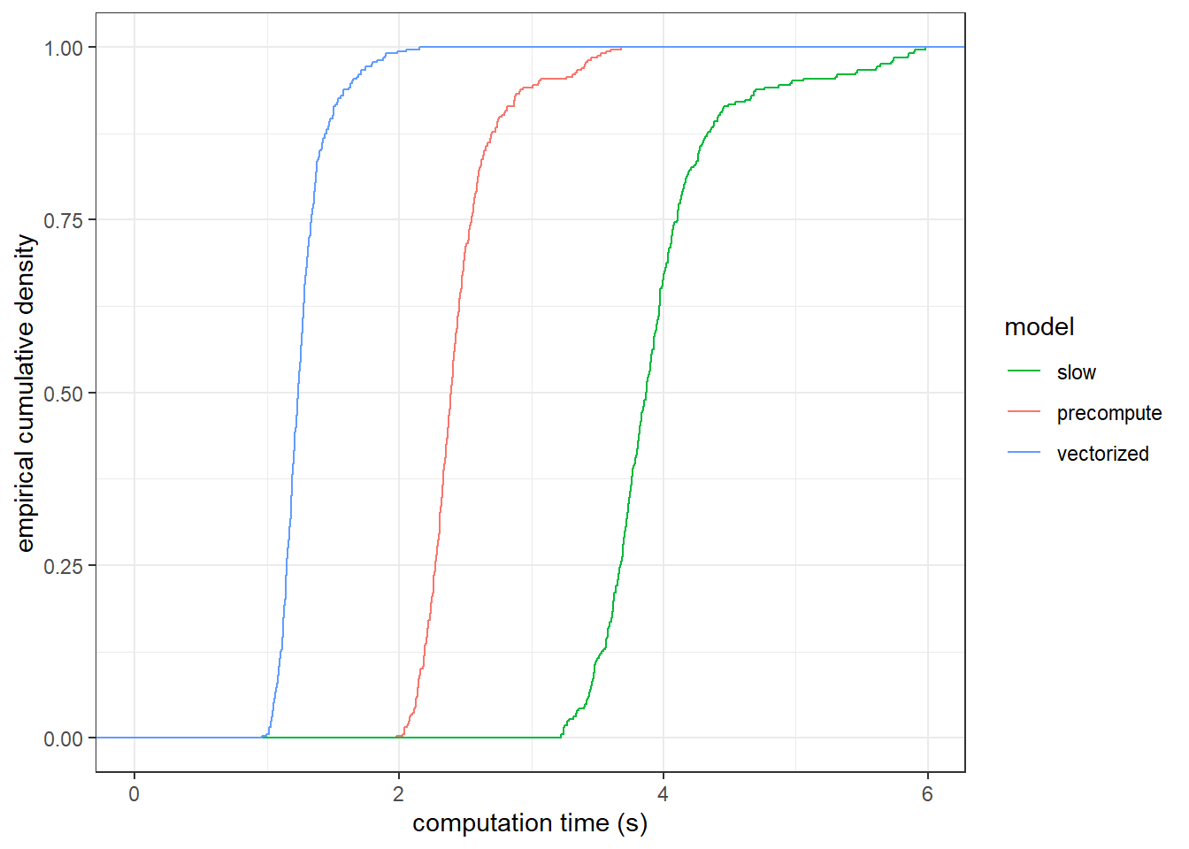
Figure 12.1: Computation time for individual-level estimation of models, excluding the paralleized program.
12.6.2 Within-chain parallelization
To evaluate the performance improvements due to within-chain paralleization, I give Stan a more difficult problem to solve. This is because there is a substantial fixed time cost associated with managing more than one core, and so there might not be much to see if we just looked at the participant-specific estimations, which only had 100 observations each. Instead, we can increase the number of things that Stan needs to add up to compute the likelihood by estimating a representative-agent model pooling all of the data. This means that instead of having to add up 100 things to compute the likelihood, Stan will need to add up 32,700 things (i.e. 327 participants each making 100 decisions).
In order to showcase the benefits of parallelization, I estimate the model with just one chain. This means that I can devote all eight cores of my server to within-chain parallelization. I estimate the model for five different values of the tuning parameter grainsize, including grainsize = 1, which allows Stan’s scheduler to determine how the sum is split up. These were chosen to roughly split the summation up into 8ths, 16ths, 32nds and so on on my 8-core server. I also estimate the model without parallelization (setting the data input doparallel to zero). The computation times are summarized in Table 12.1. For the values of grainsize explored, the computation time is about ten times faster for the parallelized process.
Parallel<-"Code/SpeedyCode/BenchmarkSummaryParallel.rds" |>
  readRDS() |>
  group_by(grainsize) |>
  summarize(
    `Time to estimate model (s)` = mean(time)
  )

Parallel |>
  round(1) |>
  kbl(caption = "Computation time for parallelized model. `grainsize = NA` indicates the un-parallelized process. `grainsize = 1` allows *Stan*'s scheduler to choose how to split up the summation.") |>
kable_classic(full_width=FALSE)| grainsize | Time to estimate model (s) |
|---|---|
| 1 | 50.9 |
| 511 | 50.1 |
| 1022 | 50.4 |
| 2044 | 56.3 |
| 4088 | 86.6 |
| NA | 539.5 |
While we should not be particularly interested in the estimates from this representative agent model, it is important to note that we can probably benefit from these improvements in other, more interesting models, too. For example if we were estimating a hierarchical model using these data, we would also need to add up 32,700 things to compute the likelihood. If we can expect similar improvements in computational time for this model, then this could turn a 3-day slog into an over-nighter!
12.7 R code to estimate models
12.7.1 Slow, pre-computed, and vectorized models
library(tidyverse)
library(haven)
library(rstan)
  rstan_options(auto_write = TRUE)
  options(mc.cores = parallel::detectCores())
  rstan_options(threads_per_chain = 8)


numreps<-1

# Note: The show-up fee for the undergrads was $10 and $40 for the MBA students

BenchmarkSummary<-tibble()

D<-"Data/HS2023.dta" |>
  read_dta() |>
  select(id,choice,prize1L:prob4R,endowment) |>
  # add in the endowment
  mutate(
    show_up_fee = ifelse(mba,40,10),
    Left = 1-choice,
    prize1L = prize1L+endowment+show_up_fee,
    prize2L = prize2L+endowment+show_up_fee,
    prize3L = prize3L+endowment+show_up_fee,
    prize4L = prize4L+endowment+show_up_fee,
    prize1R = prize1R+endowment+show_up_fee,
    prize2R = prize2R+endowment+show_up_fee,
    prize3R = prize3R+endowment+show_up_fee,
    prize4R = prize4R+endowment+show_up_fee
  ) |>
  # there were never four possible prizes
  select(-contains("4")) |>
  rowwise() |>
  mutate(
    prizerangeLow = min(c(prize1L,prize2R,prize3L)),
    prizerangeHigh = max(c(prize1L,prize2R,prize3L))
  ) |>
  filter(!is.na(Left))


ModelList<-list(
  slow = "Code/SpeedyCode/EUT_slow.stan" |> stan_model(),
  precompute = "Code/SpeedyCode/EUT_precompute.stan" |> stan_model(),
  vectorized = "Code/SpeedyCode/EUT_vectorized.stan" |> stan_model()
)


for (rr in 1:numreps) {
  for (ii  in unique(D$id)) {

    print(paste("rep",rr,"of",numreps,"id",ii,"of",length(D$id |> unique())))

    d<- D|> filter(id==ii)

    dStan<-list(
      N = dim(d)[1],
      Left = d$Left,

      prizes = cbind(d$prize1L,d$prize2L,d$prize3L),
      prizerange=cbind(d$prizerangeLow,d$prizerangeHigh),

      probL = cbind(d$prob1L,d$prob2L,d$prob3L),
      probR = cbind(d$prob1R,d$prob2R,d$prob3R),

      prior_r = c(0.27,0.36),
      prior_lambda = c(log(30),0.5)
    )

    for (mm in names(ModelList)) {

      Fit<-ModelList[[mm]] |>
        sampling(seed=42,chains=1,data=dStan,refresh=1000)

      BenchmarkSummary<- BenchmarkSummary |>
        rbind(
          tibble(id=ii,
                 model = mm,
                 rep = rr,
                 grainsize=NA,
                 time = get_elapsed_time(Fit) |> sum()
                 )
        )


    }

    BenchmarkSummary |>
      saveRDS("Code/SpeedyCode/BenchmarkSummarySeries.rds")

  }


}
12.7.2 Parallelized model
library(tidyverse)
library(haven)
library(rstan)
  rstan_options(auto_write = TRUE)
  options(mc.cores = parallel::detectCores())
  rstan_options(threads_per_chain = 8)


numreps<-10


# Note: The show-up fee for the undergrads was $10 and $40 for the MBA students

BenchmarkSummary<-tibble()

D<-"Data/HS2023.dta" |>
  read_dta() |>
  select(id,choice,prize1L:prob4R,endowment) |>
  # add in the endowment
  mutate(
    show_up_fee = ifelse(mba,40,10),
    Left = 1-choice,
    prize1L = prize1L+endowment+show_up_fee,
    prize2L = prize2L+endowment+show_up_fee,
    prize3L = prize3L+endowment+show_up_fee,
    prize4L = prize4L+endowment+show_up_fee,
    prize1R = prize1R+endowment+show_up_fee,
    prize2R = prize2R+endowment+show_up_fee,
    prize3R = prize3R+endowment+show_up_fee,
    prize4R = prize4R+endowment+show_up_fee
  ) |>
  # there were never four possible prizes
  select(-contains("4")) |>
  rowwise() |>
  mutate(
    prizerangeLow = min(c(prize1L,prize2R,prize3L)),
    prizerangeHigh = max(c(prize1L,prize2R,prize3L))
  ) |>
  filter(!is.na(Left))

GRAINSIZE<-c(1,4088,2044,1022,511)

model<-"Code/SpeedyCode/EUT_parallel.stan" |>
  stan_model()


for (rr in 1:numreps) {

    print(paste("rep",rr,"of",numreps))

    dStan<-list(
      N = dim(D)[1],
      Left = D$Left,

      prizes = cbind(D$prize1L,D$prize2L,D$prize3L),
      prizerange=cbind(D$prizerangeLow,D$prizerangeHigh),

      probL = cbind(D$prob1L,D$prob2L,D$prob3L),
      probR = cbind(D$prob1R,D$prob2R,D$prob3R),

      prior_r = c(0.27,0.36),
      prior_lambda = c(log(30),0.5),

      grainsize=1,
      doparallel = 0
    )

    Fit<-model |>
      sampling(seed=42,chains=1,data=dStan,refresh=1000)
    BenchmarkSummary<- BenchmarkSummary |>
      rbind(
        tibble(id=ii,
               model = "parallel",
               rep = rr,
               grainsize=NA,
               time = get_elapsed_time(Fit) |> sum()
        )
      )

    dStan$doparallel<-1

    for (gg in GRAINSIZE) {
      dStan$grainsize<-gg
      Fit<-model |>
        sampling(seed=42,chains=1,data=dStan,refresh=1000)

      BenchmarkSummary<- BenchmarkSummary |>
        rbind(
          tibble(id=ii,
                 model = "parallel",
                 rep = rr,
                 grainsize=gg,
                 time = get_elapsed_time(Fit) |> sum()
          )
        )

    }


    BenchmarkSummary |>
      saveRDS("Code/SpeedyCode/BenchmarkSummaryParallel.rds")


}
References
If you haven’t run one yet, what are you doing? Go back and try out some of the examples that come before this chapter!↩︎
In reality it will be a bit worse than four times faster because your computer needs to devote some time to managing the parallization. Anecdotally for me doing things on my laptop, I know that running chains in parallel on my laptop comes with a noticeable start-up time (usually 10-30 seconds) that is not present if I run the chains in series. Therefore I sometimes shut down the between-chain parallelization if each chain only takes a couple of seconds to run. This start-up time is not noticeable if I am running things on my server.↩︎