21 Application: Level-\(k\) models
In this chapter, I will show you a few ways of estimating a level-\(k\) model (Stahl and Wilson 1994) using data from a guessing game (Costa-Gomes and Crawford 2006). The level-\(k\) model is particularly useful for modeling initial play in games (or play without feedback) because it is a plausible way that participants might reason their way through their decision problem in order to choose an action.
Computationally, the model poses a slight problem for us because the parameter of interest, \(k\), is an integer, and Stan can’t cope with integer parameters. Fortunately, it is very easy (albeit somewhat slow) to estimate a model assuming a given value of \(k\). From here, we can build up a model-averaged \(k\) that has a nice interpretation. But, perhaps more satisfyingly, this really lends itself to a finite mixture model, where we estimate the distribution of \(k\) in the population. The final product also has a hierarchical specification for some nuisance parameters, which we don’t necessarily care about directly, but nevertheless have to be estimated alongside the quantities that we do care about.
21.1 Data and game
Participants in Costa-Gomes and Crawford (2006) played sixteen 2-player guessing games without feedback. In each game, player \(i\in\{1,2\}\) chose a number \(x^i\in[a^i,b^i]\).89 Their payoff functions rewarded choices that were closer to \(p^i\) multiplied by their opponent’s choice. Specifically, their payoff function was:
\[ \pi^i(x^i,x^j)=\max\{0,200-|x^i-p^ix^j|\}+\max\{0,100-|x^i-p^ix^j|/10\} \]
Note that this payoff function is single-peaked at \(x^i=p^ix^j\), where the player receives a payoff of 300.
When I got my hands on these data, one of the first things I noticed was that there was a lot of rounding of participants’ choices. Specifically, there were very few choices that were not multiples of 10. The best way for me to visualize this was to plot a histogram of the digit in the ones place of participants’ choices, which is shown in Figure 21.1:
D<-"Code/CGC2006/CGC2006cleaned.rds" |>
  readRDS() |>
  mutate(
    intchoice = choice |> round(0),
    onesplace = intchoice-10*floor(intchoice/10)
  )

(
  ggplot(D,aes(x=onesplace))
  +geom_histogram(bins=10,binwidth=1)
  +theme_bw()
  +scale_x_continuous(breaks=0:10)
  +xlab("Digit in ones place of players' choices")
)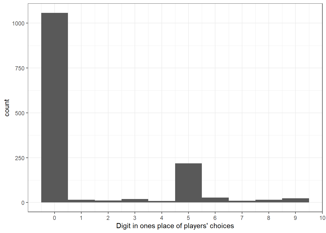
Figure 21.1: Prevalence of rounding.
This is plausible because participants in a typical game could choose between a few hundred numbers: restricting attention to just the multiples of ten probably cut out a lot of the cost of making a decision in this experiment. I therefore decided to deal exclusively with the rounded data. For example, for Game 1 player 1 has to choose a number between 100 and 500 that they think will be closest to 70% of their opponent’s choice (which must be between 100 and 900). I divide these bounds and participants’ choices by 10, round them to the nearest integer, and treat these as the data. Therefore the payoff function becomes:
\[ \pi^i(x^i,x^j)=\max\{0,200-10|x^i-p^ix^j|\}+\max\{0,100-|x^i-p^ix^j|\} \]
which means that if Player 2 chooses \(x^2=50\) (really \(x^2=500\) before dealing with rounded numbers), Player 1’s payoff function looks like this:
# payoff parameters for Player 1 in Game 1
p1<-0.7
lb1<-10
ub1<-50

# opponent's choice
x_other<-50


d<-tibble(
  # choice set
  x = seq(lb1,ub1,by=1)
) |>
  rowwise() |>
  mutate(
    u = max(c(0,200-abs(x-p1*x_other)*10))+max(c(0,100-abs(x-p1*x_other)))
  )

(
  ggplot(d,aes(x=x,y=u))
  +geom_path()
  +theme_bw()
  +ylim(c(0,300))
)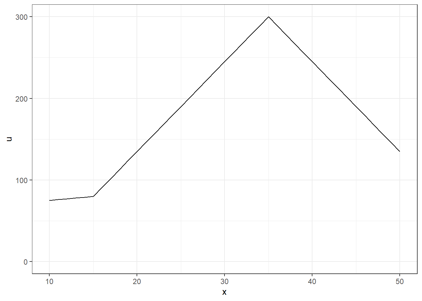
Figure 21.2: An example of a payoff function.
21.2 The level-\(k\) model
21.2.1 The deterministic component of the model
The level-\(k\) model (Stahl and Wilson 1994) is a model of introspection in games. The model assumes that there are (possibly infinite) player types (or “levels”) indexed by non-negative integers \(k=0,1,2,\ldots\). Tye level-0 type is usually assumed to randomize their action uniformly over their action space. The level-1 type best responds to the level-0 type, and so on, so that the level-\(k\) type best responds to the level-\((k-1)\) type.90
When we take a level-\(k\) model to our data, we are usually interested in estimating \(k\). That is, we want to comment on the number of steps of strategic reasoning that our participants are using.91 Since \(k\) can only take on integers, and Stan cannot deal with integer parameters, we need to be careful with how we set this up. I will walk you through a few ways of doing this. These will include Bayesian model averaging, where we estimate the model for every possible value of \(k\) under consideration, and a mixture specification, where we estimate the fraction of participants who have each value of \(k\). Whichever way seems more appealing to you, we will have to assume that participants can only be one of a finite number of possible values of \(k\). In the Bayesian model averaging case, this is because we cannot estimate “infinity” models! In the mixture model case, this is because we cannot have “infinity” behavioral types in our model. Practically in these games, as \(k\) gets large, the prediction approaches Nash equilibrium, and so at some point a \(k\) will be “large enough” that behavior should not be too different for any \(k\) larger than this. I will proceed with estimating everything assuming that \(k\leq 5\), but I have written my code so that this upper bound can be easily changed. If you’re playing along at home and your CPU has nothing better to do, all you need to do is change the kmax variable to something larger.
21.2.2 Exact and probabilistic play
The level-\(k\) model (as I have described it above) makes deterministic predictions. This is going to be a problem for our Bayesian model, as we need to have probabilistic predictions in order to write down a likelihood function. In fact, Costa-Gomes and Crawford (2006) note that a substantial fraction of their participants choose exactly according to one of their models under consideration, at least for a subset of the the games played. That is, it appears that some participants are behaving exactly according to the level-\(k\) model, and we should therefore take a model to the data that respects this kind of behavior. The solution Costa-Gomes and Crawford (2006) use, which I also adopt here, is to use a “spike logit” model, which assumes that players best respond to their belief aboth their opponent’s (possibly mixed) strategy with probability \(1-\epsilon\), and with probability \(\epsilon\) they logit respond to this belief. For the games studied here, which have relatively large action spaces, this makes for a mostly smooth probabilistic best response, except for a large mass point on the optimal action.
So how do we code this into a likelihood function? Let’s parameterize the model as \(\rho=1-\epsilon\in(0,1)\), the probability that a participant chooses their optimal action, and \(\lambda>0\), logit choice precision. Then let \(u_t(a\mid k)\) be the player’s expected utility in game \(t\) given that they are a level-\(k\) type, and \(a_t^*(k)\) is their optimal action given that they are a lvele-\(k\) type. We can then split up the likelihood contribution into two cases:
- if they choose their optimal action, then that choice could have been a best response or they just happened to logit respond with this action, or
- if they did not choose their optimal action, then they must have logit responded.
This makes our log-likelihood for an individual choice \(y_t\) in Game \(t\):
\[ \begin{aligned} \log p(y_t\mid \rho,\lambda,k)&=\begin{cases} \log\left(\rho+(1-\rho)\frac{\exp(\lambda u(y_t\mid k))}{\sum_a\exp(\lambda u(a\mid k))}\right)& \text{if } y_t = a_t^*(k)\\ \log\left((1-\rho)\frac{\exp(\lambda u(y_t\mid k))}{\sum_a\exp(\lambda u(a\mid k))}\right) & \text{otherwise} \end{cases} \end{aligned} \]
21.3 Assigning probabilities to types for each participant separately
One approach to the data, which is probably the closest in this chapter to its original treatment in Costa-Gomes and Crawford (2006), is to estimate the level-\(k\) model for each participant separately, assuming various different values of \(k\), then using some kind of model evaluation to select the value of \(k\) that best characterizes that participant. In this section, I estimate the model for each participant assuming \(k=1, 2, 3, 4, 5\), and then use Bayes factors and model averaging to determine which \(k\) best characterizes their behavior.
21.3.1 The Stan program
Here is the Stan program I came up with. Importantly, note that each level-\(k\) strategy can be pre-computed, which is going to speed things up substantially. You can see this done in the transformed data block. The predictions are stored in the arrays LKpredictions1 for player 1, and LKpredictions2 for player 2.
Another thing to note is that I am incementing the target by the full likelihood, and not just the kernel. Hence, the extensive use of target += .... This is so that we can compute the log marginal likelihood, which will be needed for model comparison.
functions {

  vector payofffun(vector x1,row_vector x2,real p1) {

    /*
    x1 is the action space of the first player

    x2 is the distribution of actions of the second player. That is, for level 0
    player 2, it is the action space (which gets averaged over a uniform
    distribution), and for level k>0 is just populated by the prediction of this
    type
    */

    int n1 = size(x1);
    int n2 = size(x2);

    matrix[n1,n2] err = fabs(rep_matrix(x1,n2)-p1*rep_matrix(x2,n1));

    vector[n1] pay = (fmax(0.0,200-err*10)+fmax(0.0,100-err))*rep_vector(1.0/n1,n2);

    return pay;


  }

  int which_max(vector x,real tol) {
    /*
    Returns the index of the vector x which corresponds to the maximum in x
    Returns the largest index if there are more than one element equal to this
    */
    int n = size(x);

    int ind = 0;

    for (ii in 1:n) {
      if (abs(x[ii]-max(x))<tol) {
        ind = ii;
      }
    }

    return ind;


  }


}

data {

  int ngames; // number of games

  int k; // level k to evaluate

  // game data
  vector[ngames] P1; // target for player 1
  vector[ngames] P2; // target for player 2
  int LB1[ngames]; // lower bound for player 1
  int UB1[ngames]; // upper bound for player 1
  int LB2[ngames]; // lower bound for player 2
  int UB2[ngames]; // upper bound for player 2

  // player 1 choice
  int choice1[ngames];

  real<lower=0> prior_probExact[2]; // Beta prior
  real prior_lambda[2]; // lognormal prior

  // tolerance for identifying a maximum in function which_max(,)
  real<lower=0> tol;


}

transformed data {

  int choice1_i[ngames];

  // pre-compute level-k predictions

  vector[k] LKpredictions1[ngames];
  vector[k] LKpredictions2[ngames];


  for (gg in 1:ngames) {
    real p1 = P1[gg];
    real p2 = P2[gg];
    int lb1 = LB1[gg];
    int ub1 = UB1[gg];
    int lb2 = LB2[gg];
    int ub2 = UB2[gg];

    int n1 = ub1-lb1+1;
    int n2 = ub2-lb2+1;

    choice1_i[gg] = choice1[gg]-lb1+1;

    // choice sets
    vector[n1] X1 = linspaced_vector(n1,lb1,ub1);
    row_vector[n2] X2 = linspaced_row_vector(n2,lb2,ub2);

    // choices to get uniform distribution over actions
    vector[n1] x1 = linspaced_vector(n1,lb1,ub1);
    row_vector[n2] x2 = linspaced_row_vector(n2,lb2,ub2);


    for (kk in 1:k) {

      vector[n1] payoff1 = payofffun(X1,x2,p1);
      vector[n2] payoff2 = payofffun(X2',x1',p2);

      x1 = rep_vector(X1[which_max(payoff1,tol)],n1);
      x2 = rep_row_vector(X2[which_max(payoff2,tol)],n2);

      LKpredictions1[gg][kk] = X1[which_max(payoff1,tol)];
      LKpredictions2[gg][kk] = X2[which_max(payoff2,tol)];
    }

  }

}


parameters {

  // probability the player chooses exactly according to the level-k model
  real<lower=0,upper=1> probExact;
  // logit choice precision for the rest of the choices
  real<lower=0> lambda;

}

model {

  for (gg in 1:ngames) {
    real p1 = P1[gg];
    real p2 = P2[gg];
    int lb1 = LB1[gg];
    int ub1 = UB1[gg];
    int lb2 = LB2[gg];
    int ub2 = UB2[gg];

    int n1 = ub1-lb1+1;
    int n2 = ub2-lb2+1;

    // choice sets for Player 1
    vector[n1] X1 = linspaced_vector(n1,lb1,ub1);

    row_vector[n2] x2;

    // action of Player 2
    if (k==1) {
      x2 = linspaced_vector(n2,lb2,ub2)';
    } else {
      x2 = rep_row_vector(LKpredictions2[gg][k-1],n2);
    }

    // Player 1 payoff
    vector[n1] payoff1 = payofffun(X1,x2,p1);

    if (choice1[gg]==LKpredictions1[gg][k]) {
    // If the choice matches exactly with the prediction, then ...
     target += log(
       probExact // best respond probability
        +(1.0-probExact)*softmax(lambda*payoff1)[choice1_i[gg]] // logit response
      );

    } else {
      // if the choice does not match exactly with the prediction, then ...
      target += log(
       (1.0-probExact)*softmax(lambda*payoff1)[choice1_i[gg]]
      );
    }

  }


  // priors
  target += beta_lpdf(probExact | prior_probExact[1],prior_probExact[2]);
  target += lognormal_lpdf(lambda | prior_lambda[1],prior_lambda[2]);


}
21.3.2 Prior calibration
The model has two parameters: \(\rho\in(0,1)\) (the probability that the player chooses their best response), and \(\lambda>0\) (logit choice precision).
As \(\rho\) is restricted to the unit interval, a Beta prior makes sense here. I ended up unsing the uniform distribution, or \(\rho\sim\mathrm{Beta}(1,1)\) for this prior.
For \(\lambda\), a log-normal distribution makes sure that the parameter is non-negative, so \(\log\lambda\sim N(m_\lambda,s_\lambda^2)\). For an idea of what might be a good choice of \(m_\lambda\) and \(s_\lambda\), let’s look at the logit response in Game 1 to player 2 choosing x_other=500 (as we did for the payoff function above in Figure 21.2).
logitResponse<-expand.grid(
  x = seq(lb1,ub1,by=1),
  lambda = c(0.01,0.02,0.05,0.1,0.2,0.5,1,2)
) |>
  rowwise() |>
  mutate(
    u = max(c(0,200-abs(x-p1*x_other)*10))+max(c(0,100-abs(x-p1*x_other)))
  ) |>
  ungroup() |>
  group_by(lambda) |>
  mutate(
    u = u-min(u),
    pr = exp(lambda*u)/sum(lambda*u),
    pr_scaled = pr/max(pr)
  )

(
  ggplot(logitResponse,aes(x=x,y=pr_scaled,color = as.factor(lambda)))
  +labs(color = expression(lambda),x = "choice",y="probability (scaled so max=1)")
  +geom_path()
  +theme_bw()
)
I then pin down the 2.5th and 97.5th percentiles of the prior with the most extreme cases of this plot:
\[ \begin{aligned} \log0.01&=m_\lambda-1.96 s_\lambda\\ \log2&=m_\lambda+1.96s_\lambda\\ 2m_\lambda&=\log0.01+\log 2\\ m_\lambda&=\frac{\log0.01+\log 2}{2}\approx-1.96\\ 2\times 1.96 s_\lambda&=\log 2-\log0.01\\ s_\lambda&=\frac{\log 2-\log0.01}{2\times1.96}\approx 1.35\\ \implies \log\lambda&\sim N(-1.96,1.35^2) \end{aligned} \]
21.3.3 Results
In this section, I estimate one model for each participant, and for each level \(k\in\{1, 2, 3, 4, 5\}\). This takes a while, but runs without any errors with RStan’s default options.92
Estimates<-"Code/CGC2006/EstimatesLevelkRepAgent.rds" |>
  readRDS()

# whoops! I forgot to add in the parameter names into the estimation code.
# Fortunately this information is stored in the rownames of the estimates
Estimates$parameter<-gsub('[[:digit:]]+', '',rownames(Estimates))


Estimates<-Estimates |>
  group_by(id,parameter) |>
  mutate(
    postprob = exp(logml-max(logml))/sum(exp(logml-max(logml))),
    meantype = sum(k*postprob),
    meanpar = sum(mean*postprob)
  )

(
  ggplot(Estimates |> filter(parameter=="probExact"),aes(x=meantype,y=meanpar))
  +geom_point()
  +xlab("Level-k type")
  +ylab("Probability of choosing exactly accorindg to the model")
  +theme_bw()
)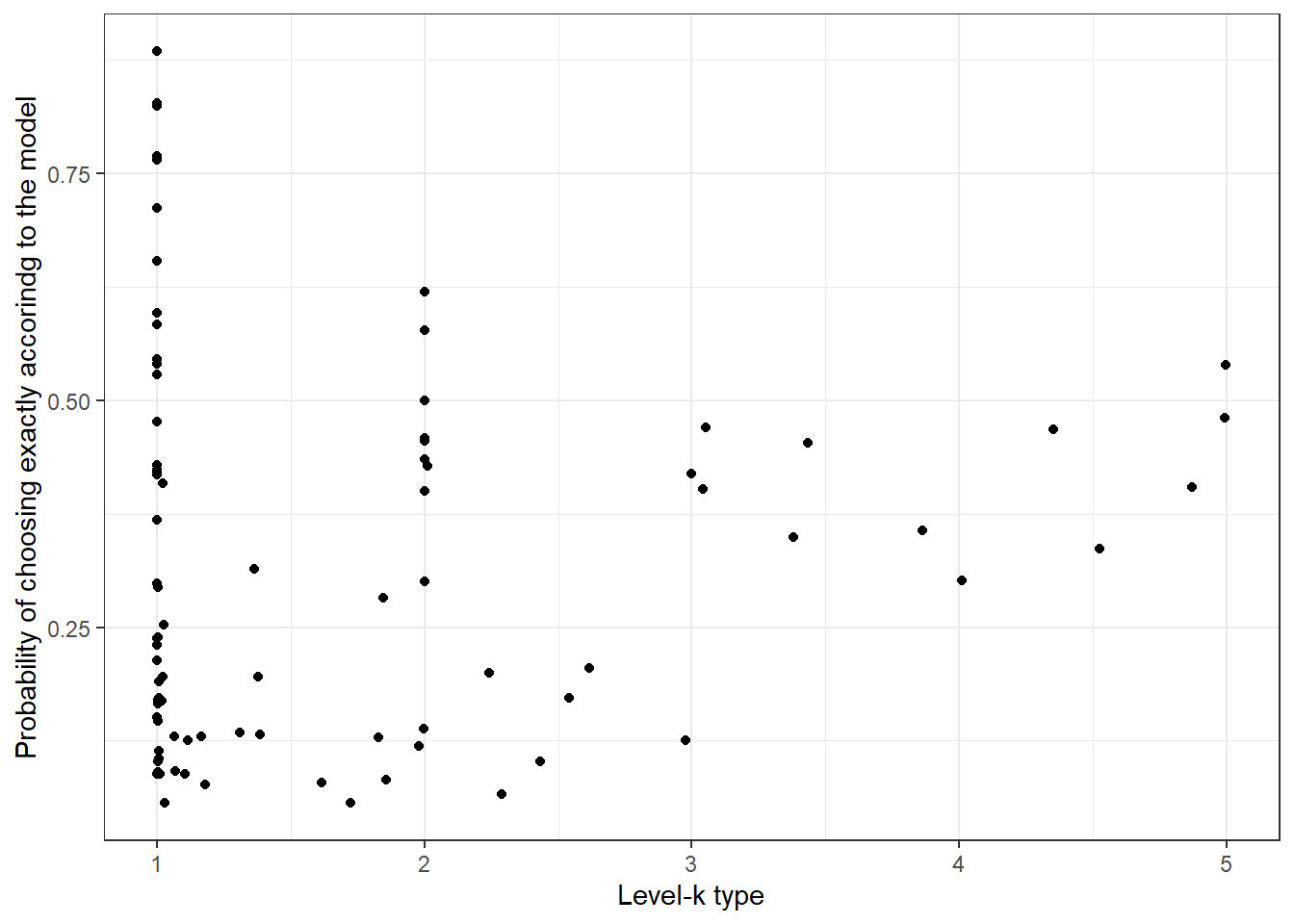
Figure 21.3: Bayesian model averages for the level-\(k\) type (horizontal axis) and the probability of choosing exactly accorindg to the model (vertical axis).
21.4 Doing the averaging within one program
The previous section provided us with a rather tedious way of estimating \(k\) for each participant: we estimated the model once for every \(k\) under consideration, then averaged over these models. While there is nothing wrong with estimating \(k\) this way, it is somewhat inefficient. To see this, note that we could have written down a model prior over the different values of \(k\), and then estimated \(\rho\) and \(\lambda\) assuming that \(k\) is drawn from this prior. To keep things simple, I will stick with a discrete uniform prior over \(k\), so that each \(k\in\{1, 2, 3, 4, 5\}\) has a 20% prior probability of being the true \(k\). Letting \(\{\psi_k\}_{k=1}^5\) be these prior probabilities, we can write the likelihood contribution for a participant’s 16 decisions as:
\[ \begin{aligned} \log p(y_t\mid \rho,\lambda)&=\log\left(\sum_{k=1}^5\psi_k\prod_{t=1}^{16}p(y_t\mid \rho,\lambda,k)\right)\\ &=\log\left(\sum_{k=1}^5\exp\left(\log \psi_k+\sum_{t=1}^{16}\log p(y_t\mid \rho,\lambda,k)\right)\right) \end{aligned} \]
This is enough information to estimate parameters \(\rho\) and \(\lambda\), but what we really care about i \(k\). So how can we go about estimating this? What we first need to do is to take our prior over \(k\), and update it based on decisions, \(\rho\), and \(\lambda\). That is, using Bayes’ rule:
\[ \begin{aligned} p(k\mid y,\rho,\lambda) &=\frac{p(y\mid k,\rho,\lambda)p(k)}{p(y\mid \rho,\lambda)}\\ &\propto p(y\mid k,\rho,\lambda)p(k)\\ \implies p(k\mid y,\rho,\lambda) &=\frac{p(y\mid k,\rho,\lambda)p(k)}{\sum_{\kappa=1}^5p(y\mid \kappa,\rho,\lambda)p(\kappa)} \end{aligned} \]
Note that we can compute everything on the right-hand side once we have posterior draws of \(\rho\) and \(\lambda\), so we can do this in the generated quantities block in Stan! The posterior means of these quantities will then be marginal posterior probabilities that we are after. That is, taking the expectation over \(\rho,\lambda\mid y\):
\[ E_{\rho,\lambda\mid y}\left[p(k\mid y,\rho,\lambda)\right] =p(k\mid y) \]
Further inspection of the final expression for \(p(k\mid y,\rho,\lambda)\) also reveals a useful similarity with our expression for the likelihood. In particular:
\[ \begin{aligned} p(y\mid k,\rho,\lambda)p(k)&=\exp(\log p(y\mid k,\rho,\lambda)+\log p(k))\\ &=\exp(\log \psi_k+\log p(y\mid k,\rho,\lambda))\\ \implies p(k\mid y,\rho,\lambda)&= \frac{\exp(\log \psi_k+\log p(y\mid k,\rho,\lambda))}{\sum_{\kappa=1}^5\exp(\log \psi_\kappa+\log p(y\mid \kappa,\rho,\lambda))} \end{aligned} \]
which is the softmax of the vector \(\{\log \psi_k+\log p(y\mid k,\rho,\lambda)\}_{k=1}^5\). All of this is to say, if we compute \(\log \psi_k+\log p(y\mid k,\rho,\lambda)\) in the transformed parameters block, we can then use it in the model block to increment the likelihood, and again in the generated quantities block to compute these posterior probabilities.
Once we have an expression for \(p(k\mid y,\rho,\lambda)\), it is straightforward to estimate \(k\) by taking the expectation in the generated quantities block. That is:
\[ E\left[k\mid y,\rho,\lambda\right]=\sum_{k=1}^5k p(k\mid y,\rho,\lambda) \]
And then the posterior mean of this will be the marginal posterior mean of \(k\), which is exactly what we are after:
\[ E[k\mid y]=E\left[E[k\mid y,\rho,\lambda]\mid y\right] \]
21.4.1 The Stan program
functions {

  vector payofffun(vector x1,row_vector x2,real p1) {

    /*
    x1 is the action space of the first player

    x2 is the distribution of actions of the second player. That is, for level 0
    player 2, it is the action space (which gets averaged over a uniform
    distribution), and for level k>0 is just populated by the prediction of this
    type
    */

    int n1 = size(x1);
    int n2 = size(x2);

    matrix[n1,n2] err = fabs(rep_matrix(x1,n2)-p1*rep_matrix(x2,n1));

    vector[n1] pay = (fmax(0.0,200-err*10)+fmax(0.0,100-err))*rep_vector(1.0/n1,n2);

    return pay;


  }

  int which_max(vector x,real tol) {

    int n = size(x);

    int ind = 0;

    for (ii in 1:n) {
      if (abs(x[ii]-max(x))<tol) {
        ind = ii;
      }
    }

    return ind;


  }


}

data {

  int ngames; // number of games

  int kmax; // max level-k to evaluate

  // game data
  vector[ngames] P1;
  vector[ngames] P2;
  int LB1[ngames];
  int UB1[ngames];
  int LB2[ngames];
  int UB2[ngames];

  // player 1 choice
  int choice1[ngames];

  real<lower=0> prior_probExact[2]; // Beta prior
  real prior_lambda[2]; // lognormal prior
  vector[kmax] prior_k; // categorical prior

  // tolerance for identifying a maximum in function which_max(,)
  real<lower=0> tol;


}

transformed data {

  int choice1_i[ngames];

  // pre-compute level-k predictions

  vector[kmax] LKpredictions1[ngames];
  vector[kmax] LKpredictions2[ngames];


  for (gg in 1:ngames) {
    real p1 = P1[gg];
    real p2 = P2[gg];
    int lb1 = LB1[gg];
    int ub1 = UB1[gg];
    int lb2 = LB2[gg];
    int ub2 = UB2[gg];

    int n1 = ub1-lb1+1;
    int n2 = ub2-lb2+1;

    choice1_i[gg] = choice1[gg]-lb1+1;

    // choice sets
    vector[n1] X1 = linspaced_vector(n1,lb1,ub1);
    row_vector[n2] X2 = linspaced_row_vector(n2,lb2,ub2);

    // choices to get uniform distribution over actions
    vector[n1] x1 = linspaced_vector(n1,lb1,ub1);
    row_vector[n2] x2 = linspaced_row_vector(n2,lb2,ub2);


    for (kk in 1:kmax) {

      vector[n1] payoff1 = payofffun(X1,x2,p1);
      vector[n2] payoff2 = payofffun(X2',x1',p2);

      x1 = rep_vector(X1[which_max(payoff1,tol)],n1);
      x2 = rep_row_vector(X2[which_max(payoff2,tol)],n2);

      LKpredictions1[gg][kk] = X1[which_max(payoff1,tol)];
      LKpredictions2[gg][kk] = X2[which_max(payoff2,tol)];
    }

  }

}


parameters {

  // probability the player chooses exactly according to the level-k model
  real<lower=0,upper=1> probExact;
  // logit choice precision for the rest of the choices
  real<lower=0> lambda;

}

transformed parameters {


  vector[kmax] like_levelk = log(prior_k);

  for (gg in 1:ngames) {
    real p1 = P1[gg];
    real p2 = P2[gg];
    int lb1 = LB1[gg];
    int ub1 = UB1[gg];
    int lb2 = LB2[gg];
    int ub2 = UB2[gg];

    int n1 = ub1-lb1+1;
    int n2 = ub2-lb2+1;

    // choice sets for Player 1
    vector[n1] X1 = linspaced_vector(n1,lb1,ub1);

    for (kk in 1:kmax) {

      row_vector[n2] x2;

      // action of Player 2
      if (kk==1) {
        x2 = linspaced_vector(n2,lb2,ub2)';
      } else {
        x2 = rep_row_vector(LKpredictions2[gg][kk-1],n2);
      }

      vector[n1] payoff1 = payofffun(X1,x2,p1);

      if (choice1[gg]==LKpredictions1[gg][kk]) {
      // If the choice matches exactly with the prediction, then ...
      like_levelk[kk] += log(
         probExact
          +(1.0-probExact)*softmax(lambda*payoff1)[choice1_i[gg]]
        );

      } else {
        // if the choice does not match exactly with the prediction, then ...
        like_levelk[kk] += log(
         (1.0-probExact)*softmax(lambda*payoff1)[choice1_i[gg]]
        );
      }

    }

  }

}

model {


  // likelihood

  target += log_sum_exp(like_levelk);


  // priors
  target += beta_lpdf(probExact | prior_probExact[1],prior_probExact[2]);
  target += lognormal_lpdf(lambda | prior_lambda[1],prior_lambda[2]);


}

generated quantities {

  vector[kmax] postprob = softmax(like_levelk);

  real postk = postprob'*linspaced_vector(kmax,1,kmax);

}
21.4.2 Results
BMA<-"Code/CGC2006/EstimatesLevelkBMA.rds" |>
  readRDS() |>
  filter(
    parameter=="probExact"
    | parameter == "lambda"
    | parameter == "postk"
  ) |>
  pivot_wider(
    id_cols=id,
    names_from = parameter,
    values_from = mean
  )

(
  ggplot(BMA,aes(x=postk,y=probExact,color = log(lambda)))
  +geom_point()
    +labs(color=expression("log("~lambda~")"))
  +theme_bw()
  +scale_color_viridis()
  +xlab("k")
  +ylab(expression(rho))
)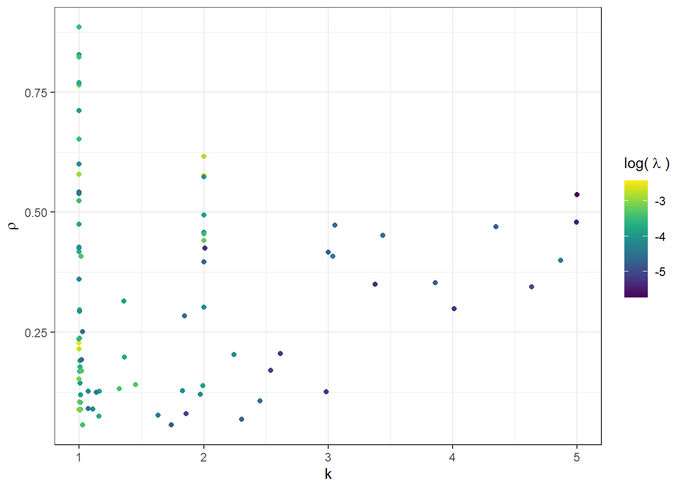
Figure 21.4: Individual-level estimates from the model assuming a discrete uniform prior over \(k\).
21.5 A mixture model
A natural extension of the participant-specific models estimated in the previous section is to use data from all participants to estimate the fraction of participants who behave according to each type. That is, the \(\psi_k\)s in the previous section are now parameters, rather than a prior, and we instead assign a prior to these new parameters. The nice product we get from this is that instead of using our flat (discrete uniform) prior over \(k\) to get our estimate of \(k\) for each participant, we now are using all of the data to get a better idea of what the fraction of types actually are in the population. Hence, if there are a lot of level-1 types in the data (which it turns out there are), then this will be reflected in our estimates of \(\psi\), and then be carried forward to our estimate of \(E[k_i\mid y_i]\).
21.5.1 Stan program
Extending the one-participant program to this one was not too difficult, but it certainly helped to have started there! The trick here was to keep track of the individual likelihoods “like_choices” in the transformed data block so that I could use them in the model block for incrementing the likelihood, and the generated quantities block for the posterior type probabilities.
functions {

  vector payofffun(vector x1,row_vector x2,real p1) {

    /*
    x1 is the action space of the first player

    x2 is the distribution of actions of the second player. That is, for level 0
    player 2, it is the action space (which gets averaged over a uniform
    distribution), and for level k>0 is just populated by the prediction of this
    type
    */

    int n1 = size(x1);
    int n2 = size(x2);

    matrix[n1,n2] err = fabs(rep_matrix(x1,n2)-p1*rep_matrix(x2,n1));

    vector[n1] pay = (fmax(0.0,200-err*10)+fmax(0.0,100-err))*rep_vector(1.0/n1,n2);

    return pay;


  }

  int which_max(vector x,real tol) {

    int n = size(x);

    int ind = 0;

    for (ii in 1:n) {
      if (abs(x[ii]-max(x))<tol) {
        ind = ii;
      }
    }

    return ind;


  }


}

data {

  int ngames; // number of games
  int nparticipants; // number of participants

  int kmax; // max level k to evaluate

  // game data
  vector[ngames] P1;
  vector[ngames] P2;
  int LB1[ngames];
  int UB1[ngames];
  int LB2[ngames];
  int UB2[ngames];

  // player 1 choice
  int choice1[nparticipants,ngames];

  vector[2] prior_probExact;
  vector[2] prior_lambda;

  vector[kmax] prior_mix;

  // tolerance for identifying a maximum in function which_max(,)
  real<lower=0> tol;


}

transformed data {

  int choice1_i[nparticipants,ngames];

  // pre-compute level-k predictions

  vector[kmax] LKpredictions1[ngames];
  vector[kmax] LKpredictions2[ngames];


  for (gg in 1:ngames) {
    real p1 = P1[gg];
    real p2 = P2[gg];
    int lb1 = LB1[gg];
    int ub1 = UB1[gg];
    int lb2 = LB2[gg];
    int ub2 = UB2[gg];

    int n1 = ub1-lb1+1;
    int n2 = ub2-lb2+1;

    for (ii in 1:nparticipants) {
      choice1_i[ii,gg] = choice1[ii,gg]-lb1+1;
    }
    // choice sets
    vector[n1] X1 = linspaced_vector(n1,lb1,ub1);
    row_vector[n2] X2 = linspaced_row_vector(n2,lb2,ub2);

    // choices to get uniform distribution over actions
    vector[n1] x1 = linspaced_vector(n1,lb1,ub1);
    row_vector[n2] x2 = linspaced_row_vector(n2,lb2,ub2);


    for (kk in 1:kmax) {

      vector[n1] payoff1 = payofffun(X1,x2,p1);
      vector[n2] payoff2 = payofffun(X2',x1',p2);

      x1 = rep_vector(X1[which_max(payoff1,tol)],n1);
      x2 = rep_row_vector(X2[which_max(payoff2,tol)],n2);

      LKpredictions1[gg][kk] = X1[which_max(payoff1,tol)];
      LKpredictions2[gg][kk] = X2[which_max(payoff2,tol)];
    }

  }

}


parameters {

  simplex[kmax] mix;

  real<lower=0,upper=1> probExact;
  real<lower=0> lambda;


}

transformed parameters {

  matrix[nparticipants,kmax] like_choices = rep_matrix(log(mix'),nparticipants);

  for (gg in 1:ngames) {
    real p1 = P1[gg];
    real p2 = P2[gg];
    int lb1 = LB1[gg];
    int ub1 = UB1[gg];
    int lb2 = LB2[gg];
    int ub2 = UB2[gg];

    int n1 = ub1-lb1+1;
    int n2 = ub2-lb2+1;

    // choice sets for Player 1
    vector[n1] X1 = linspaced_vector(n1,lb1,ub1);

    for (kk in 1:kmax) {
      row_vector[n2] x2;

      // action of Player 2
      if (kk==1) {
        x2 = linspaced_vector(n2,lb2,ub2)';
      } else {
        x2 = rep_row_vector(LKpredictions2[gg][kk-1],n2);
      }

      vector[n1] payoff1 = payofffun(X1,x2,p1);

      for (ii in 1:nparticipants) {
        if (choice1[ii,gg]==LKpredictions1[gg][kk]) {
         // If the choice matches exactly with the prediction, then ...
           like_choices[ii,kk] += log(
           probExact
              +(1.0-probExact)*softmax(lambda*payoff1)[choice1_i[ii,gg]]
            );

          } else {
      // if the choice does not match exactly with the prediction, then ...
           like_choices[ii,kk] += log(
            (1.0-probExact)*softmax(lambda*payoff1)[choice1_i[ii,gg]]
            );
          }
      } // loop over participants ends here

    } // loop over k ends here

  } // loop over games ends here


}

model {


  // priors --------------------------------------------------------------------
  mix ~ dirichlet(prior_mix);
  probExact ~ beta(prior_probExact[1],prior_probExact[2]);
  lambda ~ lognormal(prior_lambda[1],prior_lambda[2]);


  for (ii in 1:nparticipants) {
    target += log_sum_exp(like_choices[ii,]);
  }


}

generated quantities {

  matrix[nparticipants,kmax] postprob;
  vector[nparticipants] postk;

  for (ii in 1:nparticipants) {
    postprob[ii,] = softmax(like_choices[ii,]')';
    postk[ii] = postprob[ii,]*linspaced_vector(kmax,1,kmax);

  }


}
21.5.2 A prior for \(\psi\)
The parameters \(\lambda\) and \(\rho\) have the same interpretation as the previous models, so I keep their priors the same for the mixture model. The new parameter his is \(\psi\), the vector of mixing probabilities. For this, I assume:
\[ \psi\sim \mathrm{Dirichlet}(1,1,1,1,1) \]
Which means that the prior mean for each mixing probability is \(\frac{1}{5}\), and the marginal distribution of each mixing probability is:
\[ \psi_k\sim \mathrm{Beta}(1,4)\quad \forall k \]
21.5.3 Results
Mix<-summary("Code/CGC2006/EstimatesLevelkMixture.rds" |>
  readRDS()
)$summary |>
  data.frame()


Mix[c("mix[1]","mix[2]","mix[3]","mix[4]","mix[5]","probExact","lambda"),] |>
  dplyr::select(-n_eff,-Rhat) |>
  round(3) |>
  kbl(caption = "Estimates from the mixture model") |>
kable_classic(full_width=FALSE)| mean | se_mean | sd | X2.5. | X25. | X50. | X75. | X97.5. | |
|---|---|---|---|---|---|---|---|---|
| mix[1] | 0.574 | 0.001 | 0.055 | 0.465 | 0.537 | 0.575 | 0.612 | 0.680 |
| mix[2] | 0.248 | 0.001 | 0.050 | 0.158 | 0.212 | 0.246 | 0.281 | 0.352 |
| mix[3] | 0.065 | 0.000 | 0.028 | 0.021 | 0.045 | 0.062 | 0.081 | 0.128 |
| mix[4] | 0.040 | 0.000 | 0.025 | 0.005 | 0.022 | 0.036 | 0.055 | 0.101 |
| mix[5] | 0.073 | 0.000 | 0.031 | 0.023 | 0.050 | 0.069 | 0.092 | 0.145 |
| probExact | 0.331 | 0.000 | 0.013 | 0.306 | 0.323 | 0.331 | 0.340 | 0.357 |
| lambda | 0.007 | 0.000 | 0.001 | 0.006 | 0.007 | 0.007 | 0.008 | 0.009 |
Table 21.1 shows a summary of the posterior distribution of the mixture model. Here we can see that most participants are level-1, with the next most type being level 2. There seems to be a substantial spike in the probabilistic best response function, with \(\rho\) estimated to be about 0.33 (0.01).
21.6 A mixture over levels and hierarchical nuisance parameters
Up to this point, we have either estimated one model for each participant, or assumed that the parameters \(\rho\) and \(\lambda\) were constant for all participants. We can relax this with a hierarchical specification. That is, here we will preserve the mixture part of the mixture model discussed in the previous section, but add in a hierarchical specification for these parameters.
Before moving to the model specification, which at this point will not be too dissimilar from other hierarchical specifications (just with a different individual-level likelihood function), it is useful to think about why we might want to go down this route of taking participant-level heterogeneity seriously on two levels. That is, we will be assuming that participants are heterogeneous because:
- They have different levels of reasoning. That is, they have different \(k\)s, and
- They have different parameters in the probabilistic choice rule: \(\rho_i\) and \(\lambda_i\).
On the one hand, we might be interested in all of these parameters and types, and how they are different between participants. Estimating a model that allows them to be different is therefore critical for being able to comment on these things. On the other hand, and perhaps more common in the literature on level-\(k\) reasoning, we might just be interested in commenting on the distribution of \(k\) in our population, and don’t really give a hoot about \(\rho_i\) and \(\lambda_i\). In this second case, \(\rho_i\) and \(\lambda_i\) are nuisance parameters: our goal is to estimate something else, but we have to jointly estimate them in order to do this. If possible, we still want to take participant-level heterogeneity seriously here, because models that assume it away can produce misleading results (see Wilcox (2006) for a good example of this). So even though we might not want to use our estimates of \(\rho_i\) and \(\lambda_i\) to answer our research question, we want to worry about heterogeneity in these parameters.
In order to ensure the parameter restrictions for the individual-level parameters \(\lambda_i>0\) and \(\rho_i\in(0,1)\), I used the following transformed normal hierarchical specification:
\[ \theta_i\equiv\begin{pmatrix}\Phi^{-1}(\rho_i) \\ \log\lambda_i \end{pmatrix}\sim N(\mu,\mathrm{diag\_matrix}(\tau)\Omega\mathrm{diag\_matrix}(\tau)) \]
21.6.1 Prior calibration
Here we need to specify priors over the population-level parameters \(\mu\), \(\tau\), and \(\Omega\). I ended up using:
\[ \begin{aligned} \mu_\rho&\sim N(0,0.25^2)\\ \mu_\lambda&\sim N(-1.96,1.35^2)\\ \tau_\rho,\tau_\lambda &\sim \mathrm{Cauchy}^+(0,0.05)\\ \Omega&\sim \mathrm{LKJ}(4) \end{aligned} \]
For \(\mu_\lambda\), I am just using the prior I calibrated for \(\lambda\) for the participant-specific models. If anything, this is probably a bit spread out, as it seems reasonable that \(\mu_\lambda\), which pins down the median \(\lambda_i\), should be less spread out that the distribution of \(\lambda_i\) itself. For \(\mu_\rho\), we now have a probit-normal marginal distribution for \(\rho_i\), so we can’t stick with the Beta prior we had in the participant-specific models. Setting the prior mean of this parameter to 0 centers the prior median \(\rho_i\) on 50%, and a standard deviation of 0.25 means that the prior distribution is single-peaked (at \(\rho_i=50\%\)) and covers the unit interval fairly well.
21.6.2 Stan program
Here is my implementation of the hierarchical model in Stan. This took about 9 hours to run with 10,000 iterations for each of the four chains (run in parallel).93 This came as quite a relief to me, as the first Bayesian model averaging approach took over a day on the same machine!
functions {

  vector payofffun(vector x1,row_vector x2,real p1) {

    /*
    x1 is the action space of the first player

    x2 is the distribution of actions of the second player. That is, for level 0
    player 2, it is the action space (which gets averaged over a uniform
    distribution), and for level k>0 is just populated by the prediction of this
    type
    */

    int n1 = size(x1);
    int n2 = size(x2);

    matrix[n1,n2] err = fabs(rep_matrix(x1,n2)-p1*rep_matrix(x2,n1));

    vector[n1] pay = (fmax(0.0,200-err*10)+fmax(0.0,100-err))*rep_vector(1.0/n1,n2);

    return pay;


  }

  int which_max(vector x,real tol) {

    int n = size(x);

    int ind = 0;

    for (ii in 1:n) {
      if (abs(x[ii]-max(x))<tol) {
        ind = ii;
      }
    }

    return ind;


  }


}

data {

  int ngames; // number of games
  int nparticipants; // number of participants

  int kmax; // max level k to evaluate

  // game data
  vector[ngames] P1;
  vector[ngames] P2;
  int LB1[ngames];
  int UB1[ngames];
  int LB2[ngames];
  int UB2[ngames];

  // player 1 choice
  int choice1[nparticipants,ngames];

  vector[2] prior_MU[2];
  vector[2] prior_TAU;
  real prior_OMEGA;

  vector[kmax] prior_mix;

  // tolerance for identifying a maximum in function which_max(,)
  real<lower=0> tol;


}

transformed data {

  int choice1_i[nparticipants,ngames];

  // pre-compute level-k predictions

  vector[kmax] LKpredictions1[ngames];
  vector[kmax] LKpredictions2[ngames];


  for (gg in 1:ngames) {
    real p1 = P1[gg];
    real p2 = P2[gg];
    int lb1 = LB1[gg];
    int ub1 = UB1[gg];
    int lb2 = LB2[gg];
    int ub2 = UB2[gg];

    int n1 = ub1-lb1+1;
    int n2 = ub2-lb2+1;

    for (ii in 1:nparticipants) {
      choice1_i[ii,gg] = choice1[ii,gg]-lb1+1;
    }
    // choice sets
    vector[n1] X1 = linspaced_vector(n1,lb1,ub1);
    row_vector[n2] X2 = linspaced_row_vector(n2,lb2,ub2);

    // choices to get uniform distribution over actions
    vector[n1] x1 = linspaced_vector(n1,lb1,ub1);
    row_vector[n2] x2 = linspaced_row_vector(n2,lb2,ub2);


    for (kk in 1:kmax) {

      vector[n1] payoff1 = payofffun(X1,x2,p1);
      vector[n2] payoff2 = payofffun(X2',x1',p2);

      x1 = rep_vector(X1[which_max(payoff1,tol)],n1);
      x2 = rep_row_vector(X2[which_max(payoff2,tol)],n2);

      LKpredictions1[gg][kk] = X1[which_max(payoff1,tol)];
      LKpredictions2[gg][kk] = X2[which_max(payoff2,tol)];
    }

  }

}


parameters {

  simplex[kmax] mix;

  vector[2] MU;
  vector<lower=0>[2] TAU;
  cholesky_factor_corr[2] L_OMEGA;

  matrix[2,nparticipants] z;

}

transformed parameters {

  vector[nparticipants] probExact;
  vector[nparticipants] lambda;

  {

    matrix[2,nparticipants] theta = rep_matrix(MU,nparticipants)
      + diag_pre_multiply(TAU,L_OMEGA)*z;

    probExact = Phi_approx(theta[1,]');
    lambda = exp(theta[2,]');

  }


  matrix[nparticipants,kmax] like_choices = rep_matrix(log(mix'),nparticipants);

  for (gg in 1:ngames) {
    real p1 = P1[gg];
    real p2 = P2[gg];
    int lb1 = LB1[gg];
    int ub1 = UB1[gg];
    int lb2 = LB2[gg];
    int ub2 = UB2[gg];

    int n1 = ub1-lb1+1;
    int n2 = ub2-lb2+1;

    // choice sets for Player 1
    vector[n1] X1 = linspaced_vector(n1,lb1,ub1);

    for (kk in 1:kmax) {
      row_vector[n2] x2;

      // action of Player 2
      if (kk==1) {
        x2 = linspaced_vector(n2,lb2,ub2)';
      } else {
        x2 = rep_row_vector(LKpredictions2[gg][kk-1],n2);
      }

      vector[n1] payoff1 = payofffun(X1,x2,p1);

      for (ii in 1:nparticipants) {
        if (choice1[ii,gg]==LKpredictions1[gg][kk]) {
         // If the choice matches exactly with the prediction, then ...
           like_choices[ii,kk] += log(
           probExact[ii]
              +(1.0-probExact[ii])*softmax(lambda[ii]*payoff1)[choice1_i[ii,gg]]
            );

          } else {
      // if the choice does not match exactly with the prediction, then ...
           like_choices[ii,kk] += log(
            (1.0-probExact[ii])*softmax(lambda[ii]*payoff1)[choice1_i[ii,gg]]
            );
          }
      } // loop over participants ends here

    } // loop over k ends here

  } // loop over games ends here


}

model {


  // priors --------------------------------------------------------------------
  mix ~ dirichlet(prior_mix);
  for (pp in 1:2) {
    MU[pp] ~ normal(prior_MU[pp][1],prior_MU[pp][2]);
    TAU[pp] ~ cauchy(0.0,prior_TAU[pp]);
  }
  L_OMEGA ~ lkj_corr_cholesky(prior_OMEGA);

  // hierarchical structure (standardized) -------------------------------------
  to_vector(z) ~ std_normal();

  for (ii in 1:nparticipants) {
    target += log_sum_exp(like_choices[ii,]);
  }


}

generated quantities {

  matrix[2,2] OMEGA = L_OMEGA*L_OMEGA';

  matrix[nparticipants,kmax] postprob;
  vector[nparticipants] postk;

  for (ii in 1:nparticipants) {
    postprob[ii,] = softmax(like_choices[ii,]')';
    postk[ii] = postprob[ii,]*linspaced_vector(kmax,1,kmax);

  }

}
21.6.3 Results
To begin with, here are the estimates of the mixing probabilities, shown in Table 21.2. These are not too different from the mixture model assuming homogeneous \(\lambda\) and \(\rho\), but we didn’t know that before we estimated this model.
Hierarchical<- summary("Code/CGC2006/EstimatesLevelkHierarchicalMixture.rds" |>
  readRDS())$summary |>
  data.frame()


TAB<-Hierarchical[grepl("mix",rownames(Hierarchical)),]

TAB |>
  dplyr::select(-n_eff,-Rhat) |>
  round(3) |>
  kbl(caption = "Mixing probability estimates from the hierarchical/mixture level-$k$ model. ") |>
kable_classic(full_width=FALSE)| mean | se_mean | sd | X2.5. | X25. | X50. | X75. | X97.5. | |
|---|---|---|---|---|---|---|---|---|
| mix[1] | 0.604 | 0 | 0.056 | 0.493 | 0.567 | 0.605 | 0.643 | 0.711 |
| mix[2] | 0.221 | 0 | 0.048 | 0.134 | 0.189 | 0.219 | 0.252 | 0.321 |
| mix[3] | 0.069 | 0 | 0.029 | 0.023 | 0.047 | 0.066 | 0.087 | 0.134 |
| mix[4] | 0.033 | 0 | 0.023 | 0.002 | 0.016 | 0.028 | 0.045 | 0.089 |
| mix[5] | 0.073 | 0 | 0.030 | 0.024 | 0.051 | 0.069 | 0.091 | 0.142 |
Finally, we can look at the posterior means of the individual-level parameters in Figure 21.5. These are not too different from our participant-specific estimates (Figure 21.3).
Hierarchical$parameter<-gsub('[[:digit:]]+', '',rownames(Hierarchical))

d<-Hierarchical[grepl("postk",rownames(Hierarchical))
                |  grepl("probExact",rownames(Hierarchical))
                | grepl("lambda",rownames(Hierarchical))
                ,]

d$id<-parse_number(rownames(d))

d<-d |>
  pivot_wider(id_cols = id,
              names_from = "parameter",
              values_from = "mean")

(
  ggplot(d,aes(x=`postk[]`,y=`probExact[]`,color = log(`lambda[]`)))
  +geom_point()
    +labs(color=expression("log("~lambda~")"))
  +theme_bw()
  +scale_color_viridis()
  +xlab("k")
  +ylab(expression(rho))
)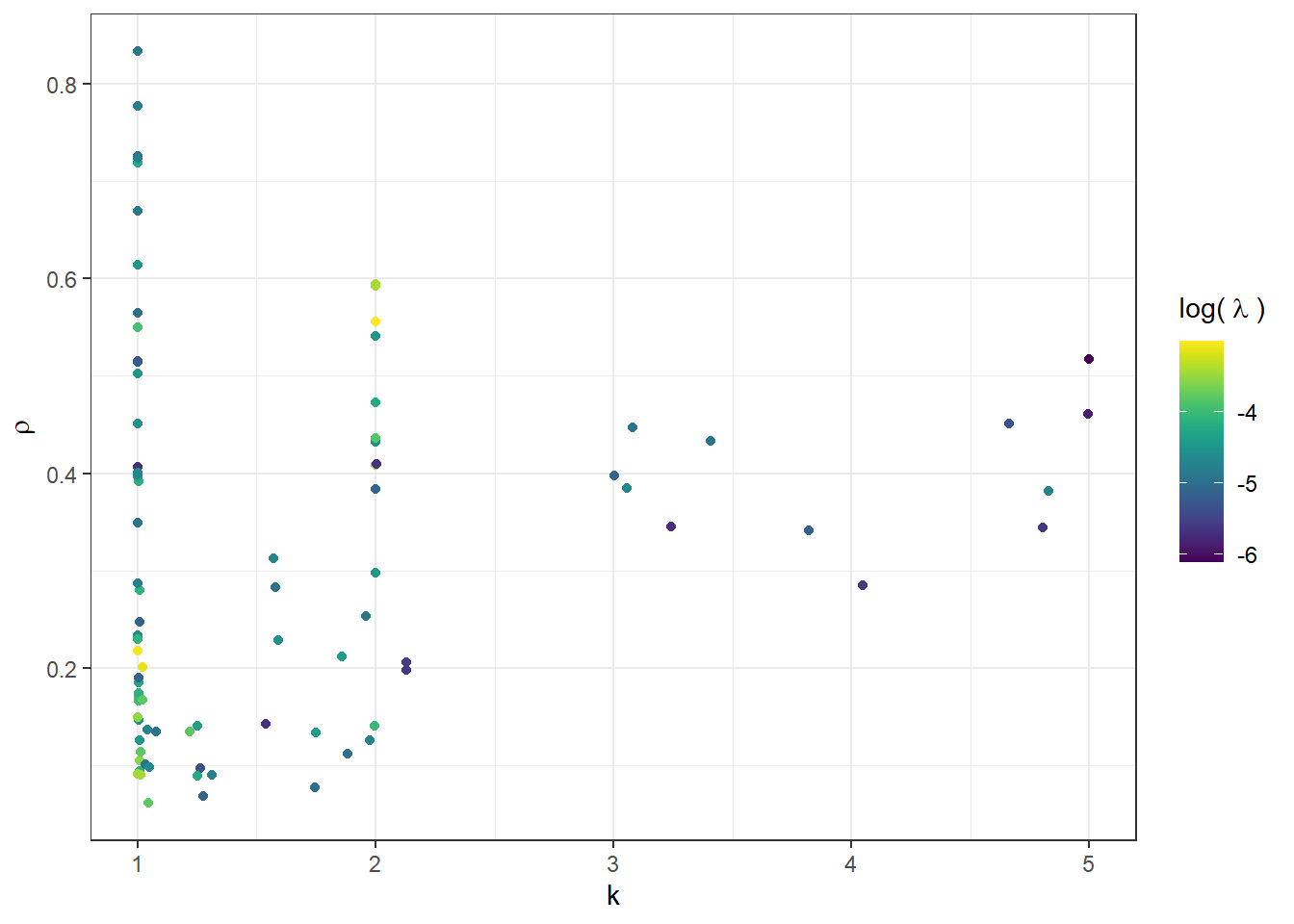
Figure 21.5: Shrinkage estimates of individual-level parameters from the heirarchical/mixture level-\(k\) model.
21.7 A different assumption about mixing
Up to this point, we maintained the simplifying assumption that a level-\(k\) type believes that they are playing against the level-\((k-1)\) prediction without any probabilistic choice. This allowed us to pre-compute the model’s deterministic predictions in the transformed data block. Here we will instead assume something much closer to the model proposed by Stahl and Wilson (1994). Specifically, we will assume that the level-\(k\) type probabilistically best responds to the aggregate mixed strategy played by all types with lower levels of strategic reasoning. That is, if each level-\(k\) type plays mixed strategy \(\sigma_k\), then this aggregate strategy that the level-\(k\) type believes is being played is:
\[ \tilde\sigma_{k-1}=\frac{\sum_{j=1}^{k-1} \psi_j\sigma_j}{\sum_{j=1}^{k-1} \psi_j} \]
That is, a level-\(k\) player’s beliefs are consistent with the true distribution of types \(\psi\), if it is truncated to only include types with lower \(k\) than the player’s.
To keep things simple here, I will drop the “spike” part of the spike-logit probabilistic choice rule (i.e. \(\rho=0\)), and assume that all participants have the same choice precision \(\lambda\). This new model is therefore most closely related to the mixture model without the hierarchical specification for \(\lambda_i\) and \(\rho_i\).94
21.7.1 Stan program
Here is the Stan file that implements this model. Note now that we have to compute the predictions in the transformed parameters block, because they are a function of \(\lambda\) and \(\psi\).
functions {

  vector logitresponse(real lambda, vector x1,row_vector x2,vector prob2,real p1) {

    /*
    x1 is the action space of the first player

    x2 is the action space of the second player

    prob2 is the mixed strategy of player 2
    */

    int n1 = size(x1);
    int n2 = size(x2);

    matrix[n1,n2] err = fabs(rep_matrix(x1,n2)-p1*rep_matrix(x2,n1));

    vector[n1] pay = lambda*(fmax(0.0,200-err*10)+fmax(0.0,100-err))*prob2;


    return softmax(pay);


  }

}

data {

  int ngames; // number of games
  int nparticipants; // number of participants

  int kmax; // max level k to evaluate

  // game data
  vector[ngames] P1;
  vector[ngames] P2;
  int LB1[ngames];
  int UB1[ngames];
  int LB2[ngames];
  int UB2[ngames];

  // player 1 choice
  int choice1[nparticipants,ngames];

  vector[2] prior_lambda;

  vector[kmax] prior_mix;

  // tolerance for identifying a maximum in function which_max(,)
  real<lower=0> tol;


}

transformed data {

  int choice1_i[nparticipants,ngames];


  for (gg in 1:ngames) {
    int lb1 = LB1[gg];

    for (ii in 1:nparticipants) {
      choice1_i[ii,gg] = choice1[ii,gg]-lb1+1;
    }


  }

}


parameters {

  simplex[kmax] mix;

  real<lower=0> lambda;


}

transformed parameters {

  matrix[nparticipants,kmax] like_choices = rep_matrix(log(mix'),nparticipants);

  for (gg in 1:ngames) {
    real p1 = P1[gg];
    real p2 = P2[gg];
    int lb1 = LB1[gg];
    int ub1 = UB1[gg];
    int lb2 = LB2[gg];
    int ub2 = UB2[gg];

    int n1 = ub1-lb1+1;
    int n2 = ub2-lb2+1;

    // choice set for Player 1
    vector[n1] X1 = linspaced_vector(n1,lb1,ub1);
    // choice set for Player 2
    vector[n2] X2 = linspaced_vector(n2,lb2,ub2);
    // level-0 strategies
    vector[n1] prob1 = rep_vector(1.0/n1,n1);
    vector[n2] prob2 = rep_vector(1.0/n2,n2);

    // aggregate strategies
    vector[n1] sigma1=prob1;
    vector[n2] sigma2=prob2;

    for (kk in 1:kmax) {

      // compute logit response to mixed strategy
      prob1 = logitresponse(lambda, X1,X2',sigma2,p1);
      prob2 = logitresponse(lambda, X2,X1',sigma1,p2);

      // add to likelihood
      like_choices[,kk] += log(prob1)[choice1_i[,gg]];

      // update mixed strategy
      if (kk == 1) {
        // aggregate strategy is the level-1 strategy
        sigma1 = prob1;
        sigma2 = prob2;
      } else {
        // aggregate strategy is a convex combination of what we had before
        // and the logit response

        sigma1 = (mix[kk]*prob1 + sum(mix[1:(kk-1)])*sigma1)/sum(mix[1:kk]);
        sigma2 = (mix[kk]*prob2 + sum(mix[1:(kk-1)])*sigma2)/sum(mix[1:kk]);


      }

    }


  } // loop over games ends here


}

model {


  // priors --------------------------------------------------------------------
  target += dirichlet_lpdf(mix | prior_mix);
  target += lognormal_lpdf(lambda | prior_lambda[1],prior_lambda[2]);


  for (ii in 1:nparticipants) {
    target += log_sum_exp(like_choices[ii,]);
  }


}


generated quantities {

  matrix[nparticipants,kmax] postprob;
  vector[nparticipants] postk;

  for (ii in 1:nparticipants) {
    postprob[ii,] = softmax(like_choices[ii,]')';
    postk[ii] = postprob[ii,]*linspaced_vector(kmax,1,kmax);

  }


}
21.7.2 Results
Estimates from this model are show in Table 21.3. Probably the most similar model for comparison is to Table 21.1. Here we have a slightly smaller fraction of level-1 types, and a more uniform distribution over the remaining types.
Eq<-summary("Code/CGC2006/EstimatesLevelkEq.rds" |>
  readRDS())$summary |>
  data.frame()

Eq |>
  filter(
    grepl("mix",rownames(Eq))
    | grepl("lambda",rownames(Eq))
  ) |>
  dplyr::select(-n_eff,-Rhat) |>
  round(3)|>
  kbl(caption = "Estimates from the mixture model assuming beliefs consistent with the truncated distribution of level-$k$ types. ") |>
kable_classic(full_width=FALSE)| mean | se_mean | sd | X2.5. | X25. | X50. | X75. | X97.5. | |
|---|---|---|---|---|---|---|---|---|
| mix[1] | 0.473 | 0.001 | 0.067 | 0.342 | 0.428 | 0.473 | 0.518 | 0.604 |
| mix[2] | 0.145 | 0.002 | 0.117 | 0.004 | 0.047 | 0.114 | 0.221 | 0.412 |
| mix[3] | 0.133 | 0.002 | 0.110 | 0.004 | 0.044 | 0.105 | 0.198 | 0.395 |
| mix[4] | 0.123 | 0.002 | 0.102 | 0.004 | 0.043 | 0.097 | 0.178 | 0.376 |
| mix[5] | 0.125 | 0.002 | 0.104 | 0.004 | 0.041 | 0.098 | 0.182 | 0.384 |
| lambda | 0.017 | 0.000 | 0.001 | 0.015 | 0.016 | 0.017 | 0.017 | 0.018 |
21.8 R code to estimate the models
21.8.1 Participant-specific estimation conditional on \(k\) with Bayesian model averaging
library(tidyverse)
library(rstan)
  rstan_options(auto_write = TRUE)
  options(mc.cores = parallel::detectCores())
library(bridgesampling)

kmax<-5

model<-"Code/CGC2006/LevelkRepAgent.stan" |>
  stan_model()

D<-"Code/CGC2006/CGC2006rounded.rds" |>
  readRDS() |>
  mutate(
    # convert choices to adjusted choices
    choice = ifelse(choice<lb1,lb1,choice),
    choice = ifelse(choice>ub1,ub1,choice)
  )

ESTIMATES<-tibble()

for (ii in unique(D$id)) {

  d<- D |> filter(id==ii)

  for (kk in 1:kmax) {

    print(paste("estimating for id",ii,"k =",kk))

    dStan<-list(

      ngames = 16,

      k = kk,

      P1 = d$p_1,
      P2 = d$p_2,
      LB1 = d$lb1,
      UB1 = d$ub1,
      LB2 = d$lb2,
      UB2 = d$ub2,

      choice1 = d$choice,

      prior_probExact = c(1,1),
      prior_lambda = c(-1.96,1.35),

      tol = 0.001


    )

    Fit<-model |>
      sampling(
        data=dStan,
        seed=42
      )

    lml<-bridge_sampler(Fit,silent=TRUE)

    ESTIMATES <- ESTIMATES |>
      rbind(
        summary(Fit)$summary |>
          data.frame() |>
          mutate(id = ii,
                 k = kk,
                 logml = lml$logml
                 )
      )
  }

  ESTIMATES |>
    saveRDS("Code/CGC2006/EstimatesLevelkRepAgent.rds")
}
21.8.2 Participant-specific estimation with a prior over \(k\)
library(tidyverse)
library(rstan)
  rstan_options(auto_write = TRUE)
  options(mc.cores = parallel::detectCores())


model<-"Code/CGC2006/LevelkBMA.stan" |>
  stan_model()

D<-"Code/CGC2006/CGC2006rounded.rds" |>
  readRDS() |>
  mutate(
    # convert choices to adjusted choices
    choice = ifelse(choice<lb1,lb1,choice),
    choice = ifelse(choice>ub1,ub1,choice)
  )


ESTIMATES<-tibble()

for (ii in unique(D$id)) {

  d<- D |> filter(id==ii)

    print(paste("estimating for id",ii))

    dStan<-list(

      ngames = 16,

      kmax = 5,

      P1 = d$p_1,
      P2 = d$p_2,
      LB1 = d$lb1,
      UB1 = d$ub1,
      LB2 = d$lb2,
      UB2 = d$ub2,

      choice1 = d$choice,

      prior_probExact = c(1,1),
      prior_lambda = c(-1.96,1.35),
      prior_k = rep(1/5,5),

      tol = 0.001


    )

    Fit<-model |>
      sampling(
        data=dStan,
        seed=42
      )

    addThis<-summary(Fit)$summary |>
      data.frame() |>
      mutate(id = ii)

    addThis$parameter<-rownames(addThis)

    ESTIMATES <- ESTIMATES |>
      rbind(addThis)

  ESTIMATES |>
    saveRDS("Code/CGC2006/EstimatesLevelkBMA.rds")
}
21.8.3 Mixture model
library(tidyverse)
library(rstan)
  rstan_options(auto_write = TRUE)
  options(mc.cores = parallel::detectCores())

model<-"Code/CGC2006/LevelkMixture.stan" |>
  stan_model()


D<-"Code/CGC2006/CGC2006rounded.rds" |>
  readRDS() |>
  arrange(id,game) |>
  mutate(
    # convert choices to adjusted choices
    choice = ifelse(choice<lb1,lb1,choice),
    choice = ifelse(choice>ub1,ub1,choice)
  )

choices<-D |>
  pivot_wider(id_cols = "id",
              names_from = game,
              values_from = choice) |>
  select(-id) |>
  as.matrix()

d<-D |> filter(id==101)


dStan<-list(
  ngames = 16,
  nparticipants = dim(choices)[1],

  kmax = 5,
  P1 = d$p_1,
  P2 = d$p_2,
  LB1 = d$lb1,
  UB1 = d$ub1,
  LB2 = d$lb2,
  UB2 = d$ub2,

  choice1 = choices,

  prior_probExact = c(1,1),
  prior_lambda = c(-1.96,1.35),

  prior_mix = rep(1,5),

  tol = 0.001


)

Fit<-model |>
  sampling(
    data=dStan,
    pars = c("like_choices"),include=FALSE,
    iter=2000,
    seed=42
      )

Fit |>
  saveRDS(file="Code/CGC2006/EstimatesLevelkMixture.rds")
21.8.4 Hierarchical model
library(tidyverse)
library(rstan)
  rstan_options(auto_write = TRUE)
  options(mc.cores = parallel::detectCores())

model<-"Code/CGC2006/LevelkHierarchicalMixture.stan" |>
  stan_model()


D<-"Code/CGC2006/CGC2006rounded.rds" |>
  readRDS() |>
  arrange(id,game) |>
  mutate(
    # convert choices to adjusted choices
    choice = ifelse(choice<lb1,lb1,choice),
    choice = ifelse(choice>ub1,ub1,choice)
  )

choices<-D |>
  pivot_wider(id_cols = "id",
              names_from = game,
              values_from = choice) |>
  select(-id) |>
  as.matrix()

d<-D |> filter(id==101)


dStan<-list(
  ngames = 16,
  nparticipants = dim(choices)[1],

  kmax = 5,
  P1 = d$p_1,
  P2 = d$p_2,
  LB1 = d$lb1,
  UB1 = d$ub1,
  LB2 = d$lb2,
  UB2 = d$ub2,

  choice1 = choices,

  prior_MU = list(
    c(0,0.25),
    c(-1.96,1.35)
  ),
  prior_TAU = c(0.05,0.05),
  prior_OMEGA = 4,
  prior_mix = rep(1,5),

  tol = 0.001


)

Fit<-model |>
  sampling(
    data=dStan,
    pars = c("z","L_OMEGA","like_choices"),include=FALSE,
    # I got the bulk and tail ESS warnings when running this with iter = 2000
    iter=10000,
    seed=42
      )

Fit |>
  saveRDS(file="Code/CGC2006/EstimatesLevelkHierarchicalMixture.rds")
21.8.5 Mixture model with beliefs consistent with truncated type distribution
library(tidyverse)
library(rstan)
  rstan_options(auto_write = TRUE)
  options(mc.cores = parallel::detectCores())

model<-"Code/CGC2006/LevelkEq.stan" |>
  stan_model()


D<-"Code/CGC2006/CGC2006rounded.rds" |>
  readRDS() |>
  arrange(id,game) |>
  mutate(
    # convert choices to adjusted choices
    choice = ifelse(choice<lb1,lb1,choice),
    choice = ifelse(choice>ub1,ub1,choice)
  )

choices<-D |>
  pivot_wider(id_cols = "id",
              names_from = game,
              values_from = choice) |>
  select(-id) |>
  as.matrix()

d<-D |> filter(id==101)


dStan<-list(
  ngames = 16,
  nparticipants = dim(choices)[1],

  kmax = 5,
  P1 = d$p_1,
  P2 = d$p_2,
  LB1 = d$lb1,
  UB1 = d$ub1,
  LB2 = d$lb2,
  UB2 = d$ub2,

  choice1 = choices,

  prior_probExact = c(1,1),
  prior_lambda = c(-1.96,1.35),

  prior_mix = rep(1,5),

  tol = 0.001


)

Fit<-model |>
  sampling(
    data=dStan,
    pars = c("like_choices"),include=FALSE,
    iter=2000,
    seed=42
      )

Fit |>
  saveRDS(file="Code/CGC2006/EstimatesLevelkEq.rds")
References
Participants in the experiment were in fact allowed to choose outside these bounds, but such choices were adjusted to the closer of the bounds. For simplicity, I describe the game in terms of these “adjusted” choices.↩︎
There are many permutations of how the level-\(k\) model is set up. I am using this one here for simplicity. Stahl and Wilson (1994), for example, assumes that the level-2 type best responds to the mixture of level-0 and level-1 types, rather than just the level-1 type. This alternative assumption is in principle implementable in both the mixture and hierarchical specifications outlined below, but would be more computationally intensive. ↩︎
We need to be careful here. A participant may be able to do many steps of strategic reasoning, but might believe that others only do a few. For example, suppose that a participant can reason their way through all of the steps (possibly infinitely many) to get to the Nash equilibrium prediction, but they believe that their opponent will make \(k=2\) steps. This participant would then behave as if they are a level-3 type. ↩︎
If you haven’t found enough shrines to get enough heart containers for the Master Sword, now is your time! This took about a day on my laptop. ↩︎
My initial run using RStan’s default 2,000 iterations per chain yielded some ESS warnings, which were easily fixed by increasing the number of iterations. ↩︎
Attempts to incorporate a hierarchical specification for \(\lambda_i\) were made, however at the time of writing there has been no joy. The added complication is that we would need to integrate out \(\lambda_i\) to compute the aggregate mixed strategy.↩︎