19 Application: QRE in a Bayesian game and cursed equilibrium
Many games we study in the lab are Bayesian games. These could include, but are not limited to, auctions, signaling games, and poker. Bayesian games involve heterogeneous players. This adds a lot of realism to the model, but also makes things more complicated, because we need to keep track of player types. For quantal response equilibrium, this usually means solving for the equilibrium mixed strategy for every type.84 Once the sytem of equations describing the QRE is set up, solving for QRE is done in exactly the same way as a non-Bayesian game.
19.1 Example game and dataset
In this chapter, we will use a game studied experimentally in Bochet and Magnani (2024). In this game, two players are randomly endowed with a quality \(q_i\in\{H,M,L\}\), and a signal \(s_i\in\{h,m,l\}\) that is informative of their opponent’s quality. Each of the three qualities are equally likely to be drawn, and players’ qualities are independent draws. After observing their qualities and signals, players play a one-shot game, whose payoffs depend on the players’ qualities. This game is shown in Table 19.1. Here \(\mu(\cdot)\) and \(\rho(\cdot)\) are funtions of qualities. In particular, note that if player \(i\) chooses to not propose (\(N\)), then they guarantee a known payoff of \(\rho(q_i)\) (since they know their own quality). They also earn this payoff if their opponent chooses \(N\), irrespective of their own action. On the other hand, if both players choose to propose (\(P\)), then each player earns a payoff that is a function of their opponent’s quality. The payoff values for \(\mu\) and \(\rho\) are shown in Table 19.2. Here there are two treatments, with Game A having a larger reservation payoff for the high type compared to Game B.
payoffs<-rbind(
  c("$\\mu(q_2)$, $\\mu(q_1)$","$\\rho(q_1)$, $\\rho(q_2)$"),
  c("$\\rho(q_1)$, $\\rho(q_2)$","$\\rho(q_1)$, $\\rho(q_2)$")
)
colnames(payoffs)<-c("P","N")->rownames(payoffs)
payoffs |>
  kbl(caption = "Proposal game studied in Bochet and Magnani (2024)") |>
kable_classic(full_width=FALSE)| P | N | |
|---|---|---|
| P | \(\mu(q_2)\), \(\mu(q_1)\) | \(\rho(q_1)\), \(\rho(q_2)\) |
| N | \(\rho(q_1)\), \(\rho(q_2)\) | \(\rho(q_1)\), \(\rho(q_2)\) |
TAB<-rbind(c(160,80,40),
           c(100,75,25),
           c(80,75,25)
           )

rownames(TAB)<-c("$\\mu(q)$","$\\rho(q)$ (Game A)","$\\rho(q)$ (Game B)")
colnames(TAB)<-c("$H$","$M$","$L$")

TAB |>
  kbl(caption = "Payoff values in game studied in Bochet and Magnani (2024)
") |>
  kable_classic(full_width=FALSE) |>
add_header_above(c(" "=1,"$q$"=3))|
\(q\)
|
|||
|---|---|---|---|
| \(H\) | \(M\) | \(L\) | |
| \(\mu(q)\) | 160 | 80 | 40 |
| \(\rho(q)\) (Game A) | 100 | 75 | 25 |
| \(\rho(q)\) (Game B) | 80 | 75 | 25 |
19.2 Solving for QRE
As in Bochet and Magnani (2024), we will here focus on the symmetric equilibrium of the game, where all players with the same type choose \(P\) with the same probability. Since there are three different qualities that a player could have, and three different signals a player could receive, this means that there are \(3\times 3=9\) types in this game. That is, the types indexed by the quality-signal combination are:
\[ (q,s)=\tau\in \{Hh,Mh,Lh, Hm, Mm, Lm, Hl, Ml, Ll\} \]
In the code below you will see that there are a lot of 9-dimensional vectors and \(9\times9\) matrices for this reason. I will use this ordering of types as a convention for indexing these vectors and matrices. For example, the fourth element of the vector of mixed strategies will correspond to the proposal probability for players who are quality \(q=H\) and receive signal \(s=m\).
We will start by deriving equations that describe the quantal response equilibrium of the game assuming that players properly condition their beliefs on whether or not their opponent proposes. This will be our “baseline” model. We will then implement a 1-parameter extension that permits players to not fully take the informational content of the opponent’s strategy into account. This is called “cursed equilibrium” (Eyster and Rabin 2005).
19.2.1 Baseline model
Note here that I am not following the notation of the original paper. I found it very helpful to work my way through this with using the joint distribution of qualities and signals, which I denote \(\pi(q,s,q',s')\). From here, all expected utilities can be expressed as a conditional distribution \(\pi(q',s'\mid q,s)\) which is a player with quality \(q\) and signal \(s\)’s belief about the quality and signal of their opponent.
A player with quality \(q\) and signal \(s\) proposes with probability \(\sigma(q,s)\). Let \(\pi(q,s)\) be the joint distribution of quality and signals.
Given signal \(s\), a player’s posterior beliefs about their opponent’s quality is:
\[ \pi(q'\mid s)=\frac{\pi(q',s)}{\pi(s)}=\frac{\pi(q',s)}{\sum_{q''}\pi(q'',s)} \]
Note that the player’s quality \(q\) is informative of the signal the opponent received. That is:
\[ \pi(s'\mid q)=\frac{\pi(q,s')}{\pi(q)}=\frac{\pi(q,s')}{\sum_{s''}\pi(q,s'')} \]
Hence, the player has informed beliefs about their opponent’s quality, \(\pi(q'\mid s)\), and informed beliefs about their opponent’s signal \(\pi(s'\mid q)\). We can summarize this as joint beliefs over the opponent’s quality and signal as follows:
\[ \begin{aligned} \pi(q',s'\mid q,s)&=\frac{\pi(q,s,q',s')}{\sum_{q',s'}\pi(q,s,q',s')} \end{aligned} \]
\[ \begin{aligned} \pi(q',s',q,s)&=\pi(s,s'\mid q,q')\pi(q,q')\\ &=\pi(s'\mid q)\pi(s\mid q')\pi(q)\pi(q') \end{aligned} \]
where the second line follows because qualities are unconditionally independent, and signals are independent conditional on opponent’s quality.85 Since \(\pi(q',s'\mid q,s)\) is only a function of the type-generating process, which is exogenous in the game, we can pre-compute these quantities in Stan’s transformed data block. You will see these computed there as PI(for the joint distribution), and PI_cond (for the conditional distribution).
It follows that the expected utility of proposing with quality \(q\) and signal \(s\) is:
\[ \begin{aligned} U^P(q,s)&=E_{q',s'}\left[\mu(q')\sigma(q',s')+(1-\sigma(q',s'))\rho(q) \mid q,s\right] \\ &=\sum_{q',s'}\left[\mu(q')\sigma(q',s')+(1-\sigma(q',s'))\rho(q)\right]\pi(q',s'\mid q,s) \end{aligned} \]
and the utility of not proposing is \(U^N(q,s)=\rho(q)\).
We can therefore write the QRE conditions in logit form, with \(\ell(q,s)=\mathrm{logit}(\sigma(q,s))\), as:
\[ \begin{aligned} H_{q,s}(\lambda,\sigma)&=\ell(q,s)-\lambda\left[\sum_{q',s'}\left[\mu(q')\sigma(q',s')+(1-\sigma(q',s'))\rho(q)\right]\pi(q',s'\mid q,s)-\rho(q)\right] \end{aligned} \]
with derivatives:
\[ \begin{aligned} \frac{\partial H_{q,s}(\lambda,\sigma)}{\partial \ell(t,v)} &=I((q,s)=(t,v))-\lambda\left[\mu(t)-\rho(q)\right]\pi(t,v\mid q,s)\frac{\partial \sigma(t,v)}{\partial \ell(t,v)}\\ &=I((q,s)=(t,v))-\lambda\left[\mu(t)-\rho(q)\right]\pi(t,v\mid q,s)\sigma(t,v)(1-\sigma(t,v)) \end{aligned} \]
and:
\[ \begin{aligned} \frac{\partial H_{q,s}}{\partial \lambda}&=-\sum_{q',s'}\left[\mu(q')\sigma(q',s')+(1-\sigma(q',s'))\rho(q)\right]\pi(q',s'\mid q,s)-\rho(q) \end{aligned} \]
I then implement a predictor-corrector algorithm as follows:86
- Initialization: Start at a known QRE. This is \(\lambda=0\), \(\sigma(q,s)=0.5\ \forall q,s\); or \(\lambda=0\), \(\ell(q,s)=0\ \forall q,s\).
- Predictor step: Use the derivative \(\frac{\partial H}{\partial \lambda}\) to predict the direction of \(\ell\) for a small increase in \(\lambda\). That is: \(\ell^{t+1}=\ell^t+\frac{\partial H}{\partial \lambda}(\lambda^{t+1}-\lambda^t)\)
- Corrector steps: Correct for any errors made with the linear approximation in (1) using Newton’s method. That is, iterate on \(\ell^{t+1}=\ell^t-\left(\frac{\partial H(\lambda,\ell)}{\partial \ell^\top}\right)^{-1}H(\lambda,\ell)\) until a desired level of accuracy is achieved.
- Repeat: If \(\lambda^t\) is less than the required \(\lambda\), go back to step (1).
Here is the Stan program I wrote to estimate this baseline QRE model. Note that I am passing an array of integers called UseData to Stan. This is a list of rows of the data that will contribute to the likelihood. This will be useful for cross-validation, as we will need to estimate the model several times leaving out different groups of observations.
functions {

  vector H(real lambda, vector ell,
    data matrix PI_cond,
    data vector mu, data vector rho,
    data int[] QQ, data int[] SS
  ) {

    vector[9] sigma = inv_logit(ell);

    vector[9] result = ell;

    for (rr in 1:9) {

      result[rr] -= lambda*(sum(
        (mu[QQ].*sigma+(1.0-sigma)*rho[QQ[rr]]).*PI_cond[,rr]
        )
        -rho[QQ[rr]]
      );

    }


    return result;

  }


  matrix DH(real lambda, vector ell,
    data matrix PI_cond,
    data vector mu, data vector rho,
    data int[] QQ, data int[] SS
  ) {
   vector[9] sigma = inv_logit(ell);

   matrix[9,9] result = diag_matrix(rep_vector(1.0,9));

   for (rr in 1:9) {
     for (cc in 1:9) {


       result[rr,cc]+= -lambda*(mu[QQ[cc]]-rho[QQ[rr]])*PI_cond[cc,rr]*sigma[cc]*(1.0-sigma[cc]);

     }
   }
   return result;
  }

  vector dlH(real lambda, vector ell,
    data matrix PI_cond,
    data vector mu, data vector rho,
    data int[] QQ, data int[] SS
  ) {

    vector[9] sigma = inv_logit(ell);

    vector[9] result = ell;

    for (rr in 1:9) {

      result[rr] -= (sum(
        (mu[QQ].*sigma+(1.0-sigma)*rho[QQ[rr]]).*PI_cond[,rr]
        )
        -rho[QQ[rr]]
      );

    }


    return result;

  }


  vector solve_QRE(real lambda,
    data matrix PI_cond,
    data vector mu, data vector rho,
    data int[] QQ, data int[] SS,
    data int maxiter, data real tol, data vector lxgrid
  ) {
       vector[9] result = rep_vector(0.0,9);

       int nx = dims(lxgrid)[1];

       for (ll in 2:nx) {

         // predictor step

         real l = lambda*0.5*(lxgrid[ll-1]+lxgrid[ll]);
         vector[9] Hlambda = dlH(l,result,PI_cond,mu,rho,QQ,SS);
         result += Hlambda*(lxgrid[ll]-lxgrid[ll-1]);

         l = lambda*lxgrid[ll];

         // corrector step
         for (ii in 1:maxiter) {

           matrix[9,9] J = DH(l,result,PI_cond,mu,rho,QQ,SS);
           vector[9]   F = H(l,result,PI_cond,mu,rho,QQ,SS);

           vector[9] dx = -J\F;

           result += dx;

           if (max(abs(dx))<tol) {

             break;
           }

           if (ii == maxiter && ll==nx) {

             print("Corrector step did not converge for lambda =",l);

           }

         }

         //
       }

       return result;
  }

}


data {

  int N;

  int<lower=1,upper=9> type[N];
  int<lower=1,upper=2> game[N];
  int<lower=0,upper=1> action[N];

  int<lower=0,upper=N> nUseData;
  int UseData[nUseData];


  vector[2] prior_lambda;

  int maxiter;
  real tol;
  int nlxgrid;

}

transformed data {

  // grid to trace out QRE

  vector[nlxgrid] lxgrid;
  for (ii in 1:nlxgrid) {
    lxgrid[ii] = (ii-1.0)/(nlxgrid-1.0);
  }


  // game parameters
  vector[3] mu = [160,80,40]';
  vector[3] rho[2];
    rho[1] = [100,75,25]';
    rho[2] = [80,75,25]';


  // data that actually contributes to the likelihood
  int type_training[nUseData] = type[UseData];
  int game_training[nUseData] = game[UseData];
  int action_training[nUseData] = action[UseData];

  // data used for testing
  int type_test[N-nUseData];
  int game_test[N-nUseData];
  int action_test[N-nUseData];

  int count_test = 1;
  int count_train = 1;
  for (ii in 1:N) {

    if (nUseData>0) {

      if (UseData[count_train]==ii) {

        if (count_train < nUseData) {
          count_train +=1;
        }

      } else {
        type_test[count_test] = type[ii];
        game_test[count_test] = game[ii];
        action_test[count_test] = action[ii];
        count_test+=1;
      }
    } else {
        type_test[count_test] = type[ii];
        game_test[count_test] = game[ii];
        action_test[count_test] = action[ii];
        count_test+=1;

    }


  }


  // some indices for identifying types


  int QQ[9];
  int SS[9];

  for (qq in 1:3) {
    for (ss in 1:3) {

      int tt = qq+3*(ss-1);

      QQ[tt] = qq;
      SS[tt] = ss;

    }
  }

  matrix[3,3] signal_likelihoods = [
    [0.5,0.5,0.0],
    [0.0,1.0,0.0],
    [0.0,0.5,0.5]
    ];

  matrix[9,9] PI;

  for (rr in 1:9) {
    for (cc in 1:9) {

      PI[rr,cc] = (1.0/3.0)*(1.0/3.0)*signal_likelihoods[QQ[rr],SS[cc]]*signal_likelihoods[QQ[cc],SS[rr]];


    }
  }

  matrix[9,9] PI_cond = rep_matrix(0.0,9,9);

  for (rr in 1:9) {
    for (cc in 1:9) {

      //if (sum(PI[,cc])>0) {
        PI_cond[rr,cc] += PI[rr,cc]/sum(PI[,cc]);
      //}

    }
  }


}


parameters {

 real<lower=0> lambda;

}

transformed parameters {

  vector[9] ELL[2];

  ELL[1] = solve_QRE(lambda,
    PI_cond,
    mu, rho[1],
    QQ,SS,
    maxiter,tol,lxgrid
  ) ;
  ELL[2] = solve_QRE(lambda,
    PI_cond,
    mu, rho[2],
    QQ,SS,
    maxiter,tol,lxgrid
  ) ;


}


model {

  // prior
  target += lognormal_lpdf(lambda | prior_lambda[1],prior_lambda[2]);

  // likelihood
  for (ii in 1:nUseData) {
    target += bernoulli_logit_lpmf(action_training[ii] |  ELL[game_training[ii]][type_training[ii]]);
  }

}

generated quantities {

  vector[9] sigma[2];
    sigma[1] = inv_logit(ELL[1]);
    sigma[2] = inv_logit(ELL[2]);

  real logL_test = 0;

  for (ii in 1:(N-nUseData)) {
    logL_test += bernoulli_logit_lpmf(action_test[ii] |  ELL[game_test[ii]][type_test[ii]]);
  }


  //matrix[9,9] PI_cond_test = PI_cond;

  //matrix[9,9] PI_test = PI;
}
19.2.2 Cursed equilibrium
In Bayesian games, a popular one-parameter extension is the “Cursed Equilibrium” (Eyster and Rabin 2005). In this model, players maintain correct beliefs about opponents’ strategies, but underestimate the information that is contained in these strategies. In this game, this means that a participant might not fully factor in that if an opponent proposes, that tells us something about their quality. In the most extreme “fully cursed” case, the player believes that their payoff if both propose is the average \(\mu(q)\) (i.e. integrating out \(q\)), which I will denote \(\bar\mu\). In the \(\chi\)-cursed model, players partially incorporate this information, and so their expected utility from proposing is:
\[ \begin{aligned} U_\chi^P(q,s)&=\sum_{q',s'}\left[\underbrace{\left((1-\chi)\mu(q')+\chi\bar \mu\right)}_\text{the new part}\sigma(q',s')-(1-\sigma(q',s'))\rho(q)\right]\pi(q',s'\mid q,s) \end{aligned} \]
where \(\chi\in[0,1]\) measures the degree of “cursedness”. Modifying the QRE equations here is relatively simple: whenever you see a \(\mu(\cdot)\), just replace it with \((1-\chi)\mu(\cdot)+\chi\bar\mu\).
Here is the Stan program I wrote to estimate the cursed model:
functions {

  vector H(real lambda, vector ell,
    real chi,
    data matrix PI_cond,
    data vector mu, data vector rho,
    data int[] QQ, data int[] SS
  ) {

    vector[9] sigma = inv_logit(ell);

    vector[9] result = ell;

    for (rr in 1:9) {

      result[rr] -= lambda*(sum(
        (((1.0-chi)*mu[QQ]+chi*mean(mu)).*sigma+(1.0-sigma)*rho[QQ[rr]]).*PI_cond[,rr]
        )
        -rho[QQ[rr]]
      );

    }


    return result;

  }


  matrix DH(real lambda, vector ell,
    real chi,
    data matrix PI_cond,
    data vector mu, data vector rho,
    data int[] QQ, data int[] SS
  ) {
   vector[9] sigma = inv_logit(ell);

   matrix[9,9] result = diag_matrix(rep_vector(1.0,9));

   for (rr in 1:9) {
     for (cc in 1:9) {


       result[rr,cc]+= -lambda*((1-chi)*mu[QQ[cc]]+chi*mean(mu)-rho[QQ[rr]])*PI_cond[cc,rr]*sigma[cc]*(1.0-sigma[cc]);

     }
   }
   return result;
  }

  vector dlH(real lambda, vector ell,
    real chi,
    data matrix PI_cond,
    data vector mu, data vector rho,
    data int[] QQ, data int[] SS
  ) {

    vector[9] sigma = inv_logit(ell);

    vector[9] result = ell;

    for (rr in 1:9) {

      result[rr] -= (sum(
        (((1.0-chi)*mu[QQ]+chi*mean(mu)).*sigma+(1.0-sigma)*rho[QQ[rr]]).*PI_cond[,rr]
        )
        -rho[QQ[rr]]
      );

    }


    return result;

  }


  vector solve_QRE(real lambda, real chi,
    data matrix PI_cond,
    data vector mu, data vector rho,
    data int[] QQ, data int[] SS,
    data int maxiter, data real tol, data vector lxgrid
  ) {
       vector[9] result = rep_vector(0.0,9);

       int nx = dims(lxgrid)[1];

       for (ll in 2:nx) {

         // predictor step

         real l = lambda*0.5*(lxgrid[ll-1]+lxgrid[ll]);
         vector[9] Hlambda = dlH(l,result,chi,PI_cond,mu,rho,QQ,SS);
         result += Hlambda*(lxgrid[ll]-lxgrid[ll-1]);

         l = lambda*lxgrid[ll];

         // corrector step
         for (ii in 1:maxiter) {

           matrix[9,9] J = DH(l,result,chi,PI_cond,mu,rho,QQ,SS);
           vector[9]   F = H(l,result,chi,PI_cond,mu,rho,QQ,SS);

           vector[9] dx = -J\F;

           result += dx;

           if (max(abs(dx))<tol) {

             break;
           }

           if (ii == maxiter && ll==nx) {

             print("Corrector step did not converge for lambda =",l);

           }

         }

         //
       }

       return result;
  }

}


data {

  int N;

  int<lower=1,upper=9> type[N];
  int<lower=1,upper=2> game[N];
  int<lower=0,upper=1> action[N];

  int<lower=0,upper=N> nUseData;
  int UseData[nUseData];


  vector[2] prior_lambda;
  vector[2] prior_chi;

  int maxiter;
  real tol;
  int nlxgrid;

}

transformed data {

  // grid to trace out QRE

  vector[nlxgrid] lxgrid;
  for (ii in 1:nlxgrid) {
    lxgrid[ii] = (ii-1.0)/(nlxgrid-1.0);
  }


  // game parameters
  vector[3] mu = [160,80,40]';
  vector[3] rho[2];
    rho[1] = [100,75,25]';
    rho[2] = [80,75,25]';


  // data that actually contributes to the likelihood
  int type_training[nUseData] = type[UseData];
  int game_training[nUseData] = game[UseData];
  int action_training[nUseData] = action[UseData];

  // data used for testing
  int type_test[N-nUseData];
  int game_test[N-nUseData];
  int action_test[N-nUseData];

  int count_test = 1;
  int count_train = 1;
  for (ii in 1:N) {

    if (nUseData>0) {

      if (UseData[count_train]==ii) {

        if (count_train < nUseData) {
          count_train +=1;
        }
      } else {
        type_test[count_test] = type[ii];
        game_test[count_test] = game[ii];
        action_test[count_test] = action[ii];
        count_test+=1;
      }
    } else {
        type_test[count_test] = type[ii];
        game_test[count_test] = game[ii];
        action_test[count_test] = action[ii];
        count_test+=1;

    }


  }


  // some indices for identifying types


  int QQ[9];
  int SS[9];

  for (qq in 1:3) {
    for (ss in 1:3) {

      int tt = qq+3*(ss-1);

      QQ[tt] = qq;
      SS[tt] = ss;

    }
  }

  matrix[3,3] signal_likelihoods = [
    [0.5,0.5,0.0],
    [0.0,1.0,0.0],
    [0.0,0.5,0.5]
    ];

  matrix[9,9] PI;

  for (rr in 1:9) {
    for (cc in 1:9) {

      PI[rr,cc] = (1.0/3.0)*(1.0/3.0)*signal_likelihoods[QQ[rr],SS[cc]]*signal_likelihoods[QQ[cc],SS[rr]];


    }
  }

  matrix[9,9] PI_cond = rep_matrix(0.0,9,9);

  for (rr in 1:9) {
    for (cc in 1:9) {

      //if (sum(PI[,cc])>0) {
        PI_cond[rr,cc] += PI[rr,cc]/sum(PI[,cc]);
      //}

    }
  }


}


parameters {

 real<lower=0> lambda;
 real<lower=0,upper=1> chi;

}

transformed parameters {

  vector[9] ELL[2];

  ELL[1] = solve_QRE(lambda,chi,
    PI_cond,
    mu, rho[1],
    QQ,SS,
    maxiter,tol,lxgrid
  ) ;
  ELL[2] = solve_QRE(lambda,chi,
    PI_cond,
    mu, rho[2],
    QQ,SS,
    maxiter,tol,lxgrid
  ) ;


}


model {

  // prior
  target += lognormal_lpdf(lambda | prior_lambda[1],prior_lambda[2]);
  target += beta_lpdf(chi | prior_chi[1],prior_chi[2]);

  // likelihood
  for (ii in 1:nUseData) {
    target += bernoulli_logit_lpmf(action_training[ii] |  ELL[game_training[ii]][type_training[ii]]);
  }

}

generated quantities {

  vector[9] sigma[2];
    sigma[1] = inv_logit(ELL[1]);
    sigma[2] = inv_logit(ELL[2]);

  real logL_test = 0;

  for (ii in 1:(N-nUseData)) {
    logL_test += bernoulli_logit_lpmf(action_test[ii] |  ELL[game_test[ii]][type_test[ii]]);
  }

}
19.3 A quick prior calibration
The cursed model has two parameters: \(\lambda>0\) and \(\chi\in(0,1)\). For \(\chi\) I am going to assume a uniform prior, meaning that in the prior each level of cursedness is equally likely. I do this because the parameter has natural bounds, and we don’t want to rule out or favor any particular values of \(\chi\). On the other hand, I found it much harder to think about a prior for \(\lambda\). Without looking at the model’s predictions, it is hard to have any idea what values of \(\lambda\) seem reasonable. So we will do just that: look at the predictions. To do this, I traced out the QRE mixed strategies for a wide range of \(\lambda\) using Stan’s Fixed_param algorithm. Here are what the predictions look like for the baseline model (\(\chi=0\)):
QRE<-"Code/BM2024/QRE.csv" |>
  read.csv() |>
  mutate(
    quality = paste("quality =",quality) |> factor(levels = paste("quality =",c("H","M","L")) ),
    signal = paste("signal =",signal) |> factor(levels = paste("signal =",c("h","m","l")) )
  )

 (
    ggplot(QRE,aes(x=lambda,y=sigma,linetype=game))
    +facet_grid(quality~signal)
    +geom_line()
    +scale_x_continuous(trans="log10")
    +theme_bw()
    +xlab(expression(lambda))
    +ylab(expression(sigma~(proposal~rate)))
  )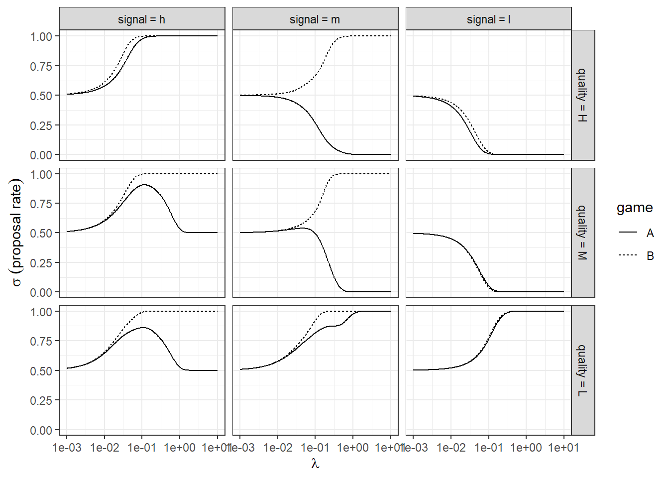
Figure 19.1: QRE predictions for the baseline (\(\chi=0\)) model.
Looking at Figure 19.1, I noticed that (i) play is effectively coin-flipping for \(\lambda<10^{-3}\), and (ii) play appears to have converged for \(\lambda>1\). I will deem this the “interesting” part of the QRE correspondence, and place 95% prior probability in this region. That is, if we use a log-normal prior \(\log\lambda\sim N(m,s^2)\), then:
\[ \begin{aligned} \log(10^{-3})&=m-1.96s\\ \log(1)&=m+1.96s\\ \log(10^{-3})+\log(1)&=2m\\ m&=\frac{1}{2}(\log(10^{-3})+\log(1))\approx-3.45\\ \log(1)-\log(10^{-3})&=2\times 1.96s\\ s&=\frac{\log(1)-\log(10^{-3})}{2\times 1.96}\approx1.76 \end{aligned} \]
Which, for another sanity check, gets us a prior median for \(\lambda\) of \(\exp(-3.45)\approx 0.032\) and prior mean of \(\exp(-3.45+0.5\times 1.76^2)\approx0.149\).
19.4 Model results
Here are Stan’s summaries of the models’ parameters:
Fit_baseline<- summary("Code/BM2024/Fit_baseline_qre.rds" |>
  readRDS())$summary |>
  data.frame() |>
  rownames_to_column(var = "parameter") |>
  filter(parameter=="lambda" | parameter=="chi") |>
  mutate(model = "baseline") |>
  dplyr::select("model","parameter","mean","se_mean","sd","X2.5.","X25.","X50.","X75.","X97.5.","n_eff","Rhat")

Fit_cursed<-summary("Code/BM2024/Fit_cursed_qre.rds" |>
  readRDS())$summary |>
  data.frame() |>
  rownames_to_column(var = "parameter") |>
  filter(parameter=="lambda" | parameter=="chi") |>
  mutate(model = "cursed") |>
  dplyr::select("model","parameter","mean","se_mean","sd","X2.5.","X25.","X50.","X75.","X97.5.","n_eff","Rhat")

TAB<-rbind(Fit_baseline,Fit_cursed) |>
  mutate(
    parameter = paste0("$\\",parameter,"$")
  )

TAB |>
  kbl(digits=3,caption = "Summary of the two models' posterior distributions") |>
kable_classic(full_width=FALSE) | model | parameter | mean | se_mean | sd | X2.5. | X25. | X50. | X75. | X97.5. | n_eff | Rhat |
|---|---|---|---|---|---|---|---|---|---|---|---|
| baseline | \(\lambda\) | 0.091 | 0.000 | 0.004 | 0.083 | 0.088 | 0.091 | 0.094 | 0.099 | 1124.232 | 1.001 |
| cursed | \(\lambda\) | 0.097 | 0.000 | 0.004 | 0.090 | 0.095 | 0.097 | 0.100 | 0.105 | 3600.401 | 1.000 |
| cursed | \(\chi\) | 0.350 | 0.001 | 0.030 | 0.289 | 0.330 | 0.351 | 0.371 | 0.406 | 3454.873 | 1.000 |
So we can be fairly certain that \(\chi\in(0.2,0.4)\) for the cursed model.87
Interpreting \(\chi\) is something we can do. \(\chi\approx0.35\) is closer to the baseline model than full cursedness, but it is still substantially far away from zero. So we should conclude that players are substantially cursed, but not fully cursed.
It is also useful with QRE to look at what they say about choices. To do this, I plot the posterior distributions of the mixed strategy alongside the empirical frequencies of actions in the experiment. These are shown in Figures 19.2 and 19.3. Firstly, it looks like the cursed model does slightly better at matching the data than does the baseline model. We will be a bit more rigorous in the next section with a model evaluation. But what I really like about these models is that they are organizing the data very well for just one or two parameters! The cursed model only has two parameters, but it is making predictions about eighteen empirical choice frequencies.
predictions_cursed<-extract("Code/BM2024/Fit_cursed_qre.rds" |>
  readRDS())$sigma

predictions_baseline<-extract("Code/BM2024/Fit_baseline_qre.rds" |>
  readRDS())$sigma

quality<-rep(c("H","M","L"),3)
signal<-c(rep("h",3),rep("m",3),rep("l",3))

PREDICTIONS<-tibble()

for (tt in 1:9) {
  for (gg in 1:2) {

    PREDICTIONS<-rbind(
      PREDICTIONS,
      tibble(
        game = c("A","B")[gg],type=tt,model="baseline",
        sigma = predictions_baseline[,gg,tt]
      ),
      tibble(
        game = c("A","B")[gg],type=tt,model="cursed",
        sigma = predictions_cursed[,gg,tt]
      )
      )

  }
}

PREDICTIONS<-PREDICTIONS |>
  mutate(
    quality = quality[type],
    signal = signal[type]
  ) |>
  mutate(
    quality = paste("quality =",quality) |> factor(levels = paste("quality =",c("H","M","L")) ),
    signal = paste("signal =",signal) |> factor(levels = paste("signal =",c("h","m","l")) )
  )

min_round<-21

empirical<-"Data/BochetMagnani2024/data_analysis/data/Main_data_base_game.csv" |>
  read.csv() %>%
  filter(subsession.round_number>=min_round) %>%
  mutate(player.type=factor(player.type)) %>%
  mutate(player.type=fct_recode(player.type,
                                "H"="1",
                                "M"="2",
                                "L"="3")) %>%
  mutate(player.signal=factor(player.signal)) %>%
  mutate(player.signal=fct_recode(player.signal,
                                  "h"="1",
                                  "m"="2",
                                  "l"="3")) %>%
  mutate(subsession.game_name=factor(subsession.game_name)) |>
  # now for JB's but coding up things to pass to Stan --------------------------
  mutate(
    type_code = paste0(player.type,player.signal) |>
      factor(levels = c("Hh","Mh","Lh","Hm","Mm","Lm","Hl","Ml","Ll")) |>
      as.numeric(),

    game_code = ifelse(subsession.game_name=="A",1,2),

    action = player.choice,

    uid = participant.code |> factor() |> as.numeric(),

    ugroupid = paste(session.code,group.id_in_subsession) |> factor() |> as.numeric()
  ) |>
  ungroup() |>
  mutate(
    rownum = 1:n()
  )|>
  group_by(player.type,player.signal,game_code) |>
  summarize(
    `Proposal rate` = mean(action)
  ) |>
  mutate(
    quality = paste("quality =",player.type) |> factor(levels = paste("quality =",c("H","M","L")) ),
    signal = paste("signal =",player.signal) |> factor(levels = paste("signal =",c("h","m","l")) )
  )


(
  ggplot(PREDICTIONS |> filter(game=="A"),aes(x=sigma,fill=model))
  +geom_histogram(aes(y=after_stat(density)),bins=100)
  +geom_vline(data=empirical |> filter(game_code==1),aes(xintercept=`Proposal rate`))
  +facet_grid(quality~signal)
  +theme_bw()
  +xlab(expression(sigma~(proposal~rate)))
  +ylab("posterior density")
  +scale_fill_manual(values = c("blue","red"))
  +labs(title = "Game A")
)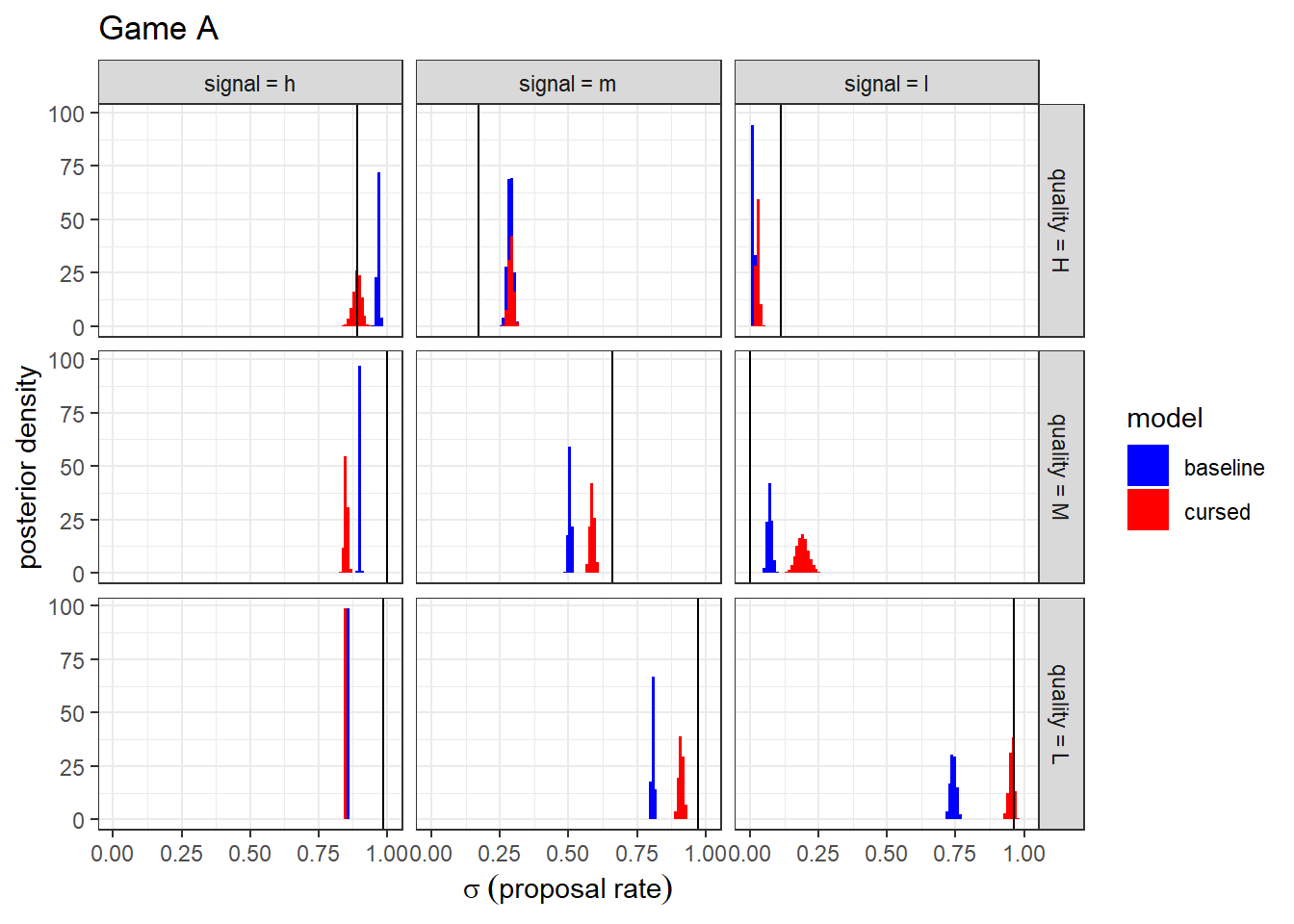
Figure 19.2: Posterior distribution of mixed strategies (histograms) and empirical choice frequencies (vertical black lines) for Game A
(
  ggplot(PREDICTIONS |> filter(game=="B"),aes(x=sigma,fill=model))
  +geom_histogram(aes(y=after_stat(density)),bins=100)
  +geom_vline(data=empirical |> filter(game_code==2),aes(xintercept=`Proposal rate`))
  +facet_grid(quality~signal)
  +theme_bw()
  +xlab(expression(sigma~(proposal~rate)))
  +ylab("posterior density")
  +scale_fill_manual(values = c("blue","red"))
  +labs(title = "Game B")
)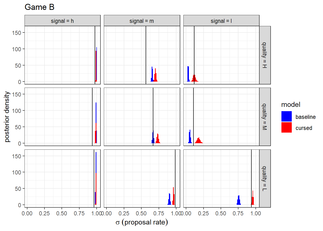
Figure 19.3: Posterior distribution of mixed strategies (histograms) and empirical choice frequencies (vertical black lines) for Game B
19.5 Model evaluation
Since we have taken two models to the data, we should do some kind of model evaluation to see which model we should work with. Here, I divided up the data into the six independent groups of participants (they were randomly re-matched within these groups) and performed 6-fold cross-validation based on these groups. Using ELPD as the measure of out-of-sample goodness-of-fit, it looks like the cursed model performs better here.
## [1] -811.7324## [1] -758.262719.6 R code used in this chapter
library(tidyverse)
library(rstan)
rstan_options(auto_write = TRUE)
options(mc.cores = parallel::detectCores())

RERUN<-FALSE

# Here I am following the replication package in importing the data -----------

# set min round ---------------------------------------------------
min_round <- 21

D<-"Data/BochetMagnani2024/data_analysis/data/Main_data_base_game.csv" |>
  read.csv() %>%
  filter(subsession.round_number>=min_round) %>%
  mutate(player.type=factor(player.type)) %>%
  mutate(player.type=fct_recode(player.type,
                                "H"="1",
                                "M"="2",
                                "L"="3")) %>%
  mutate(player.signal=factor(player.signal)) %>%
  mutate(player.signal=fct_recode(player.signal,
                                  "h"="1",
                                  "m"="2",
                                  "l"="3")) %>%
  mutate(subsession.game_name=factor(subsession.game_name)) |>
  # now for JB's but coding up things to pass to Stan --------------------------
  mutate(
    type_code = paste0(player.type,player.signal) |>
      factor(levels = c("Hh","Mh","Lh","Hm","Mm","Lm","Hl","Ml","Ll")) |>
      as.numeric(),

    game_code = ifelse(subsession.game_name=="A",1,2),

    action = player.choice,

    uid = participant.code |> factor() |> as.numeric(),

    ugroupid = paste(session.code,group.id_in_subsession) |> factor() |> as.numeric()
  ) |>
  ungroup() |>
  mutate(
    rownum = 1:n()
  )

# My attempt to replicate Figure 5

dplt<-D |>
  filter(game_code==1) |>
  group_by(player.type,player.signal) |>
  summarize(
    `Proposal rate` = mean(action)
  )

(
  ggplot(dplt,aes(x=player.type,y=`Proposal rate`,fill = player.signal))
  +geom_bar(stat="identity", position=position_dodge())
)

# and Figure 6

dplt<-D |>
  filter(game_code==2) |>
  group_by(player.type,player.signal) |>
  summarize(
    `Proposal rate` = mean(action)
  )

(
  ggplot(dplt,aes(x=player.type,y=`Proposal rate`,fill = player.signal))
  +geom_bar(stat="identity", position=position_dodge())
)


# I'm happy with that

dStan<-list(
  N = dim(D)[1],

  type = D$type_code,
  game = D$game_code,
  action = D$action,

  nUseData = 0,
  UseData = array(dim=0),

  prior_lambda = c(-3.45,1.76),

  maxiter = 100,
  tol = 1e-6,
  nlxgrid = 100
)


model<-"Code/BM2024/baseline_qre.stan" |>
  stan_model()

cursed_model<-"Code/BM2024/cursed_qre.stan" |>
  stan_model()

# Check that the thing works


Fit<-model |>
  sampling(data=dStan,chains=1,iter=10,
           algorithm = "Fixed_param",init = list(list(lambda = 1))
           )
# trace out a grid of lambda to get the QRE correspondence
file<-"Code/BM2024/QRE.csv"

if (!file.exists(file) | RERUN) {
  QRE<-tibble()

  for (lambda in  (0.001*10^seq(0,4,by=0.01))) {

    Fit<-model |>
      sampling(data=dStan,chains=1,iter=1,
               algorithm = "Fixed_param",init = list(list(lambda = lambda))
      )

    SIGMA<-extract(Fit)$sigma[1,,]

    QRE<-rbind(QRE,
               tibble(
                 lambda = lambda,
                 sigma1=SIGMA[1,],
                 sigma2=SIGMA[2,],
                 logL = extract(Fit)$logL_test
               )|>
                 mutate(type=1:n())
               )

  }

  quality<-rep(c("H","M","L"),3)
  signal<-c(rep("h",3),rep("m",3),rep("l",3))

  QRE<-QRE |>
    mutate(
      quality = quality[type],
      signal = signal[type]
    ) |>
    pivot_longer(
      cols = sigma1:sigma2,
      names_to = "var",
      values_to="sigma"
    ) |>
    mutate(
      game = c("A","B")[var |> parse_number()]
    )

  QRE |>
    write.csv(file)

  (
    ggplot(QRE,aes(x=lambda,y=sigma,linetype=game))
    +facet_grid(quality~signal)
    +geom_line()
    +scale_x_continuous(trans="log10")
    +theme_bw()
    +xlab(expression(lambda))
    +ylab(expression(sigma))
  )

  plotThis<-QRE |>
    filter(game=="A",quality=="H",signal=="h")

  (
    ggplot(plotThis,aes(x=lambda,y=logL))
    +geom_line()
    +scale_x_continuous(trans="log10")
    +theme_bw()
    +coord_cartesian(ylim = c(-3000,0))
  )

}
# Estimate the baseline model

file<-"Code/BM2024/Fit_baseline_qre.rds"

if (!file.exists(file) | RERUN) {
  print("fitting baseline model")
  dStan<-list(
    N = dim(D)[1],

    type = D$type_code,
    game = D$game_code,
    action = D$action,

    nUseData = dim(D)[1],
    UseData = D$rownum,#UseData = array(dim=0),

    prior_lambda = c(-3.45,1.76),

    maxiter = 100,
    tol = 1e-3,
    nlxgrid = 100
  )

  Fit<-model |>
    sampling(data=dStan,chains=4,iter=2000,
             seed=42
    )

  Fit |>
    saveRDS(file)

}


# Estimate the baseline model

file<-"Code/BM2024/Fit_cursed_qre.rds"

if (!file.exists(file) | RERUN) {
  print("fitting cursed model")
  print("https://www.youtube.com/watch?v=CI1-74VQgUk")
  dStan<-list(
    N = dim(D)[1],

    type = D$type_code,
    game = D$game_code,
    action = D$action,

    nUseData = dim(D)[1],
    UseData = D$rownum,

    prior_lambda = c(log(0.1),1),
    prior_chi = c(1,1),

    maxiter = 100,
    tol = 1e-3,
    nlxgrid = 100
  )

  Fit<-cursed_model |>
    sampling(data=dStan,chains=4,iter=2000,
             seed=42
    )

  Fit |>
    saveRDS(file)

}

# k-fold CV --------------------------------------------------------------------

file<-"Code/BM2024/kfoldCV.rds"

if (!file.exists(file) | RERUN) {

  ll_baseline<-c()
  ll_cursed<-c()

  for (gg in sort(unique(D$ugroupid))) {

    print(paste("estimating leaving out group",gg))

    UseData<-D |>
      filter(ugroupid!=gg)

    dStan<-list(
      N = dim(D)[1],

      type = D$type_code,
      game = D$game_code,
      action = D$action,

      nUseData = dim(UseData)[1],
      UseData = UseData$rownum,

      prior_lambda = c(-3.45,1.76),
      prior_chi = c(1,1),

      maxiter = 100,
      tol = 1e-3,
      nlxgrid = 100
    )

    print("     Estimating baseline model")

    Fit_baseline<-model |>
      sampling(data=dStan,chains=4,iter=2000,
               seed=42
      )

    print("     Estimating cursed model")

    Fit_cursed<-cursed_model |>
      sampling(data=dStan,chains=4,iter=2000,
               seed=42
      )


    ll_baseline<-cbind(ll_baseline,extract(Fit_baseline)$logL)
    ll_cursed<-cbind(ll_cursed,extract(Fit_cursed)$logL)
  }

  list(
    baseline = ll_baseline,
    cursed = ll_cursed
  ) |>
    saveRDS(file)

}
References
There are some Bayesian games where we need not do this. These are games where an opponent’s type does not affect the player’s utility function. See James R. Bland (2023b) for more details on this.↩︎
Think about how you would simulate qualities and signals here. You would (1) draw each player’s quality, then (2) use this to draw their opponent’s signal. ↩︎
This is a variant on the predictor-corrector algorithm discussed earlier in this book. Here, I fix a grid of \(\lambda\)s, with the last \(\lambda\) being the value we need to compute QRE, and trace out the QRE over this grid.↩︎
I want to make it clear here that I am not trying to exactly replicate Table 9 of Bochet and Magnani (2024), who estimate \(\chi\approx 0.9\) for the games. My estimation just uses data from the games, whereas they include data from two other tasks.↩︎