8 Filling in the blanks: Imputation
Sometimes our data don’t tell us much, if anything, about the parameters we would like to estimate. If this is the case in general, then there is not much we can do about it. On the other hand, if this is only a problem for specific participants, then something is salvageable.
For example, consider the hierarchical model we took to the Bruhin, Fehr, and Schunk (2019) dictator game data. In this, there were two parameters of interest: aversion to disadvantageous inequality \(\alpha_i\) and aversion to advantageous inequality \(\beta_i\) (assuming we were not interested in choice precision \(\lambda_i\)). What if for some (but not all) participants, we didn’t have any data to identify \(\beta_i\), but we still needed to estimate it? That is, all we have for these subjects are our posterior draws of \(\alpha_i\) and \(\lambda_i\). Fortunately, our hierarchical model will naturally fill in the blanks. The reason it can do this is because the hierarchical model has an understanding of the underlying population distribution of \(\begin{pmatrix}\alpha_i & \beta_i & \lambda_i \end{pmatrix}^\top\), and can use this to make an informed guess about all of the individual-level parameters, even if there is no information in the likelihood about specific individual-level parameters. At the very least it can fill in the blanks with the marginal population means. But if there is information about some of the individual-level parameters in the likelihood, and our assumption about the population distribution permits it, it can also use this information to make a more precise estimate of the missing parameter.
8.1 Example model and dataset: yet again with Bruhin, Fehr, and Schunk (2019)
To fix ideas, let’s have a quick refresher on my favorite example dataset: the Bruhin, Fehr, and Schunk (2019) dictator game data. Here, we will again be trying to estimate the inequality-aversion model of Fehr and Schmidt (1999), which for two people is:
\[ \begin{aligned} U_i(x,y)&=x-\alpha_i\underbrace{\max\{0,y-x\}}_{\text{disadvantageous inequality}}-\beta_i\underbrace{\max\{0,x-y\}}_{\text{advantageous inequality}} \end{aligned} \]
Furthermore, as with all of the other applications so far, I will assume a logit probabilistic choice rule with precision parameter \(\lambda_i\).
d1<-(read.csv("Data/BFS2019_choices_exp1.csv")
     |> mutate(experiment=1)
)
d2<-(read.csv("Data/BFS2019_choices_exp2.csv")
     |> mutate(experiment=2)
)
D<-(rbind(d1,d2)
    # Just use the dictator game data
    |> filter(dg==1)
    |> mutate(
      self_alloc = ifelse(choice_x==1,self_x,self_y),
      other_alloc = ifelse(choice_x==1,other_x,other_y)
    )
) |>
  mutate(
    domain.x = ifelse(self_x>other_x,"adv","disadv"),
    domain.y = ifelse(self_y>other_y,"adv","disadv"),
    domain = ifelse(domain.x == "adv" & domain.y == "adv","advantageous inequality",
                            ifelse(domain.x == "disadv" & domain.y == "disadv","disadvantageous inequality",
                            "mixed")
                            )
  ) |>
  filter(sid==sid[1])

(
  ggplot(D,aes(x=self_x,y=other_x,xend=self_y,yend=other_y,color=domain))
  +geom_segment()
  +theme_bw()
  +coord_fixed()
  +xlab("Payoff to self")
  +ylab("Payoff to other")
  +geom_abline(slope=1,intercept=0,color="black",linetype="dashed")
)
Figure 8.1: Choices presented to participants in Bruhin, Fehr, and Schunk (2019). Each line segment represents a binary choice, where the two allocations are the endpoints of the line segment. Black dashed line is a \(45^\circ\) line.
Figure 8.1 shows the choices presented to participants in this dictator game task. Importantly here, I have divided up the choices (represented by line segments) into three “domains” (represented by colors). First, the green line segments represent choices that were made exclusively in the disadvantageous inequality domain. For these choices, the payoff to the other person is always greater than the payoff to the self. If we only had these data to work with, we could only reliably estimate \(\alpha_i\) and \(\lambda_i\). Next, the red line segments show choices that were made exclusively in the advantageous inequality domain. That is, all of these choices had the self earning more than the other. If all we had were data from these choices, we would only be able to identify \(\beta_i\) and \(\lambda_i\). Finally, the blue line segments all cut the \(45^\circ\) line, and are therefore mixed. That is, for one option the self earns more than the other, and for the other option the other earns more than the self. For these choices, we could reasonably identify all of the parameters.
For this exercise, I will assume that we don’t have all of the data. Specifically, for the first half of the participants in the data, I will throw out all decisions made in the advantageous inequality (red) and mixed (blue) domains. Therefore we will not have any information in their data about parameter \(\beta_i\). As you will see, though, if we appropriately construct the hierarchical model, that does not mean that there is no information about their \(\beta_i\) in other participants’ data.
8.2 How is this going to work?
Consider again the individual-level estimates of \(\alpha_i\) and \(\beta_i\) from the hierarchical models chapter (specifically the estimates from the hierarchical model with an explicit correlation matrix \(\Omega\) assumed in the specification). I reproduce these posterior mean estimates in Figure 8.2.
AllData<-"Code/ImputingStuff/00_run_alldata.csv" |>
  read.csv() |>
  filter(
    grepl("alpha",par) | grepl("beta",par) | grepl("lambda", par)
  ) |>
  mutate(
    id = parse_number(par),
    parameter = gsub("[^A-Za-z]", "", par)
  ) |>
  pivot_wider(
    id_cols = id,
    names_from = parameter,
    values_from = mean
  )

(
  ggplot(AllData, aes(x=alpha,y=beta,color=log(lambda)))
  +geom_point()
  +scale_color_viridis()
  +theme_bw()
  +xlab(expression(alpha[i]~"(posterior mean)"))
  +ylab(expression(beta[i]~"(posterior mean)"))
)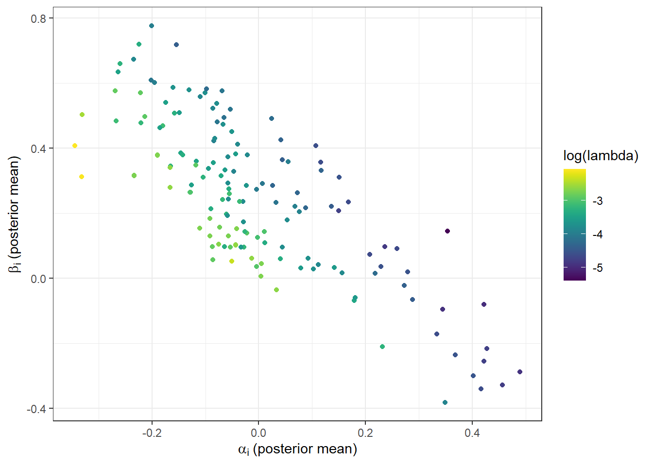
Figure 8.2: Posterior means of the individual-level parameters from the hierarchical model using the full dataset and a correlation matrix
Suppose I showed you this plot, and told you that another participant had an \(\alpha_i=-0.2\). How could you use this plot to get an estimate of \(\beta_i\)? Well, a good first pass would be to look at the posterior means in this plot that were close to the horizontal coordinate of \(\alpha_i=-0.2\) and pick out a vertical coordinate near these points (say, about \(\beta_i=0.6\)). Loosely here you are conditioning your estimate of \(\beta_i\) on \(\alpha_i\). That is, you are taking advantage of the known correlation between \(\alpha_i\) and \(\beta_i\) to note that the distribution \(\beta_i\mid\alpha_i\) is much more precise than just the marginal distribution of \(\beta_i\) (i.e. conditional on nothing). In other words, you can do better than just guessing the population mean of \(\beta_i\) by exploiting the correlation between \(\alpha_i\) and \(\beta_i\). In fact, if I had given you one, you could also have used an estimate of \(\lambda_i\). For example it looks like greater values of \(\lambda_i\) are associated with smaller values of \(\beta_i\), so this could be something else you could condition on.
What we are doing here is using our understanding of the correlation between the parameters to get a better estimate of \(\beta_i\) by conditioning on some things that we know. However this is not necessarily the norm for hierarchical models at the moment. Formally, when we go to estimate our model, we need to allow our model to take advantage of that correlation. By this, I mean that we need to actually have a correlation matrix in our hierarchical model.34
8.3 Implementation
Here the implementation is almost exactly the same as the hierarchical model I already took to these data (with the demand for giving bit in the generated quantities block taken out). Instead, we just feed it different data (i.e. taking out half of the mixed and advantageous inequality decisions). But in order to demonstrate the heavy lifting that the correlation matrix is doing for this task, I wanted to have a Stan program that could estimate a model both with and without a correlation matrix. Here is that program, where the UseCorr data variable turns on or off the use of the correlation matrix:
data {
  int<lower=0> n; // number of observations
  vector[n] self_x; // payoff to self with allocation x
  vector[n] other_x; // payoff to other with allocation x
  vector[n] self_y; // payoff to self with allocation y
  vector[n] other_y; // payoff to other with allocation y
  array[n] int choice_x; // =1 iff allocation x is chosen

  array[n] int id;
  int nParticipants;


  vector[2] prior_mu[3];
  real prior_tau[3];
  real prior_LKJ;

  int UseCorr; // >0 iff we are using the correlation matrix


}

transformed data {
  vector[n] dX; // disadvantageous inequality at allocation x
  vector[n] dY; // disadvantageous inequality at allocation y
  vector[n] aX; // advantageous inequality at allocation X
  vector[n] aY; // advantageous inequality at allocation X

  dX = fmax(0,other_x-self_x);
  dY = fmax(0,other_y-self_y);
  aX = fmax(0,self_x-other_x);
  aY = fmax(0,self_y-other_y);


}
parameters {

  vector[3] mu; // population mean
  vector<lower=0>[3] tau; // population standard deviation
  cholesky_factor_corr[3] L_Omega; // Cholesky factorization of the correlation matrix

  matrix[3,nParticipants] z; // standard normals determinig participants' parameters

}

transformed parameters {

  vector[nParticipants] alpha;
  vector[nParticipants] beta;
  vector[nParticipants] lambda;

  {
    matrix[3,nParticipants] theta;


    if (UseCorr>0) {
      // if we are using the correlation matrix

      theta = mu*rep_row_vector(1.0,nParticipants)
                    +diag_pre_multiply(tau,L_Omega)*z;
    } else {
      // if we are not using the correlation matrix
      theta = mu*rep_row_vector(1.0,nParticipants)
                    +diag_matrix(tau)*z;
    }

    alpha  = theta[1,]';
    beta   = theta[2,]';
    lambda = exp(theta[3,]');
  }

}
model {

  vector[n] Ux; // utility of allocation x
  vector[n] Uy; // utility of allocation y


  Ux = self_x-alpha[id] .* dX-beta[id] .* aX;
  Uy = self_y-alpha[id] .* dY-beta[id] .* aY;


  choice_x ~ bernoulli_logit(lambda[id] .* (Ux-Uy));

  to_vector(z) ~ std_normal();

  for (pp in 1:3) {
    mu[pp] ~ normal(prior_mu[pp][1],prior_mu[pp][2]);
    tau[pp] ~ cauchy(0.0,prior_tau[pp]);
  }

   L_Omega ~ lkj_corr_cholesky(prior_LKJ);
}

generated quantities {
  matrix[3,3] Omega;
  Omega = L_Omega*L_Omega';

}
8.4 Results
8.4.1 Using the correlation matrix
First, I estimate the model with the correlation matrix. This model is able to extrapolate estimates beyond their marginal population means. Figure 8.3 shows the individual posterior means for \(\alpha_i\) and \(\beta_i\) for the missing data (imputed for \(\beta_i\), blue) and not missing data (red).35 While there is quite a lot of overlap between these two slices of the data, one noticeable difference is that the blue (imputed) dots are pulled to the center vertically. This is to be expected, as they are shrinkage estimates. In particular, since there is no information about \(\beta_i\) in the likelihood for these subjects there is more shrinkage to the mean.36
dcorr<-"Code/ImputingStuff/00_run_leaveout_corr.csv" |>
  read.csv() |>
  mutate(
    data = "missing"
  )|>
  filter(
    grepl("alpha",par) | grepl("beta",par) | grepl("lambda", par)
  ) |>
  ungroup() |>
  mutate(
    id = parse_number(par),
    parameter = gsub("[^A-Za-z]", "", par)
  ) |>
  pivot_wider(
    id_cols = id,
    names_from = parameter,
    values_from = mean
  ) |>
  mutate(
    imputed = ifelse(id<=(n()/2),"yes","no")
  )

(
  ggplot(dcorr, aes(x=alpha,y=beta,color=imputed))
  +geom_point()
  +scale_color_manual(values=c("red","blue"))
  +theme_bw()
  +xlab(expression(alpha[i]~"(posterior mean)"))
  +ylab(expression(beta[i]~"(posterior mean)"))
)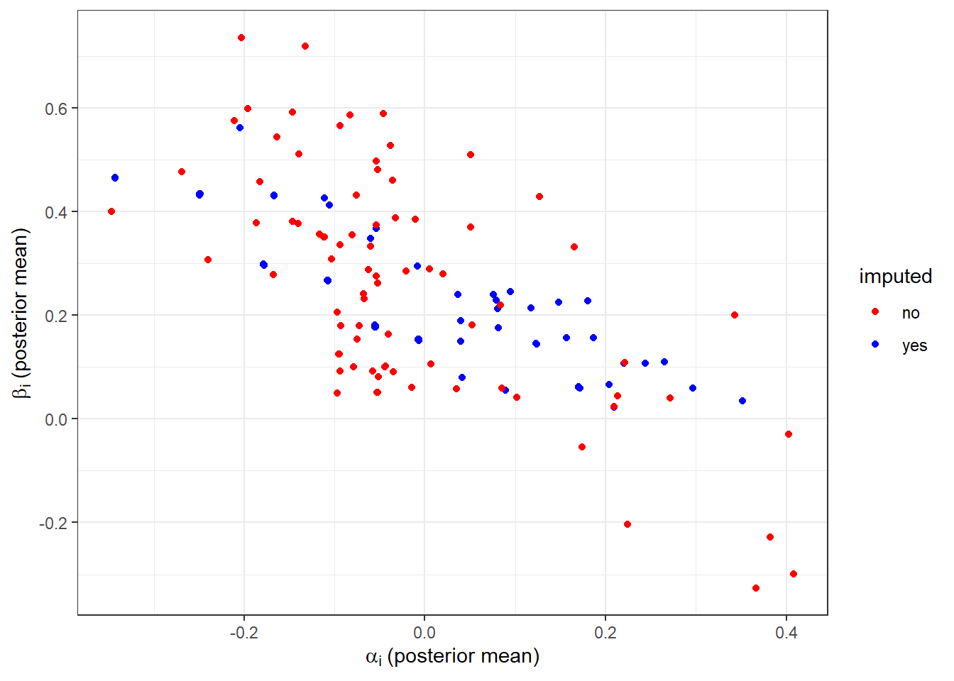
Figure 8.3: Posterior mean estimates of individual-level parameters using data with missing mixed and advantageous inequality participants.
Next, I do something that we can only do because we actually have the full dataset. In Figure 8.4 I compare the estimates of \(\beta_i\) from the data with missing observations (vertical coordinate) to the same estimates when the full dataset is used (horizontal coordinate). Here we can see that the red posterior means, which correspond to participants whose observations were not dropped, are in very strong agreement. On the other hand, the imputed \(\beta_i\)s are, understandably, shrunk toward their population mean vertically. Again, this is a feature of the model: we are using the population quantities \(\mu\), \(\tau\), and \(\Omega\) to get better estimates of \(\beta_i\) when there is no information in the likelihood for these participants. Here we can see a general upward trend, meaning that participants with larger \(\beta_i\)s are typically imputed as such, but there is substantial noise.
dcorr<-"Code/ImputingStuff/00_run_leaveout_corr.csv" |>
  read.csv() |>
  mutate(
    data = "missing"
  ) |>
  rbind(
    "Code/ImputingStuff/00_run_alldata.csv" |>
      read.csv() |>
      mutate(
        data = "full"
      )
  ) |>
  filter(
    grepl("alpha",par) | grepl("beta",par) | grepl("lambda", par)
  ) |>
  mutate(
    id = parse_number(par),
    parameter = gsub("[^A-Za-z]", "", par)
  )  |>
  filter(parameter == "beta") |>
  pivot_wider(
    id_cols = id,
    names_from = data,
    values_from = mean
  ) |>
  mutate(
    imputed = ifelse(id<=(n()/2),"yes","no")
  )


(
  ggplot(dcorr,aes(x=full,y=missing,color=imputed))
  +geom_point()
  +scale_color_manual(values=c("red","blue"))
  +theme_bw()
  +geom_abline(slope=1, intercept=0,linetype="dashed")
  +xlab(expression(beta[i]~"estimated using full dataset (posterior means)"))
  +ylab(expression(beta[i]~"estimated with missing data (posterior means)"))
)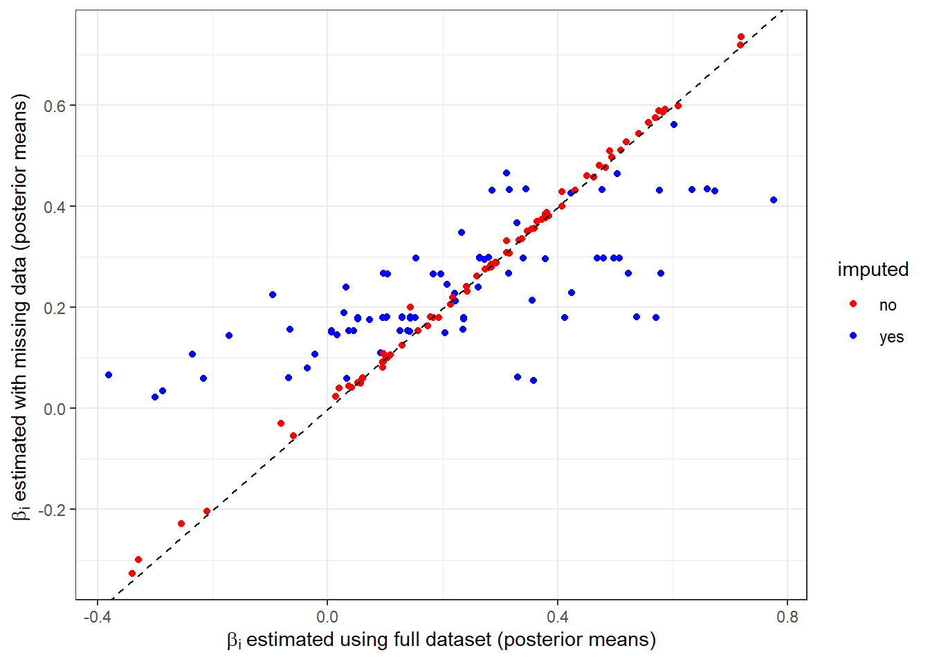
Figure 8.4: Comparison between estimates of \(\beta_i\) using the full dataset (horizontal coordinate) to those using the dataset with missing data (vertical coordinate). Dashed black line is a \(45^\circ\) line.
Of course, looking just at the posterior means masks any sense of uncertainty we have in these estimates, and there is a lot of uncertainty. Fortunately, since we have a full posterior simulation, it is easy to investigate that uncertainty as well. Figure 8.5 plots the kernel-smoothed density of the individual-level posterior standard deviations. Here we can see that especially for \(\beta_i\) (middle panel), the imputed posteriors (blue) are much more spread out than those that had an informative likelihood (red). This is to be expected because we have less information for these observations.
dcorr<-"Code/ImputingStuff/00_run_leaveout_corr.csv" |>
  read.csv() |>
  mutate(
    data = "missing"
  )|>
  filter(
    grepl("alpha",par) | grepl("beta",par) | grepl("lambda", par)
  ) |>
  ungroup() |>
  mutate(
    id = parse_number(par),
    parameter = gsub("[^A-Za-z]", "", par)
  ) |>
  mutate(
    imputed = ifelse(id<=(max(id)/2),"yes","no")
  )

(
  ggplot(dcorr,aes(x=sd,color=imputed))
  +geom_density(linewidth=1)
  +facet_wrap(~parameter,labeller = label_parsed)
  +theme_bw()
  +scale_color_manual(values=c("red","blue"))
  +xlab("posterior standard deviation")

)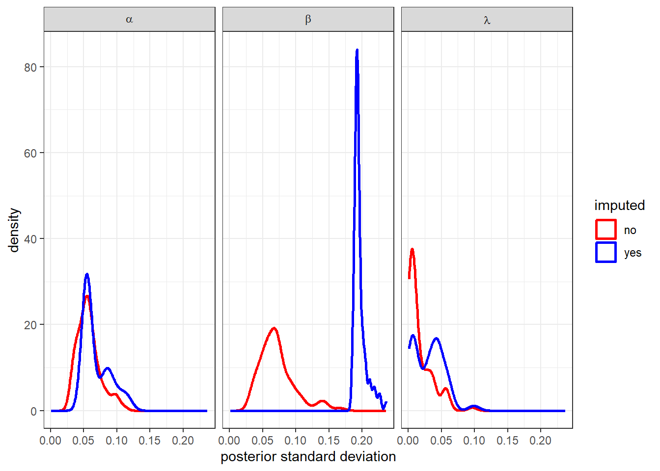
Figure 8.5: Distribution of posterior standard deviations of individual-level parameters from the model with a corelation matrix, leaving out half of the decisions in the mixed and advantageous inequality domains.
8.4.2 The correlation matrix is doing a lot of heavy lifting here
So what happens if we leave out the correlation matrix? This is why in my Stan program above I added the UseCorr data variable so it could easily be turned on or off. In this case, the model has no understanding of the correlation between the individual-level parameters. In fact, it has a lot of understanding, but that understanding is wrong. It knows dogmatically that there is no correlation between these parameters! Therefore, it is going to ignore all the information we give it about \(\alpha_i\) and \(\lambda_i\) when trying to impute \(\beta_i\), because according to the model there is nothing we could possibly learn about \(\beta_i\) from these other parameters.
d<-"Code/ImputingStuff/00_run_leaveout_nocorr.csv" |>
  read.csv() |>
  mutate(
    data = "missing"
  )|>
  filter(
    grepl("alpha",par) | grepl("beta",par) | grepl("lambda", par)
  ) |>
  ungroup() |>
  mutate(
    id = parse_number(par),
    parameter = gsub("[^A-Za-z]", "", par)
  ) |>
  pivot_wider(
    id_cols = id,
    names_from = parameter,
    values_from = mean
  ) |>
  mutate(
    imputed = ifelse(id<=(n()/2),"yes","no")
  )

(
  ggplot(d, aes(x=alpha,y=beta,color=imputed))
  +geom_point()
  +scale_color_manual(values=c("red","blue"))
  +theme_bw()
  +xlab(expression(alpha[i]~"(posterior mean)"))
  +ylab(expression(beta[i]~"(posterior mean)"))
)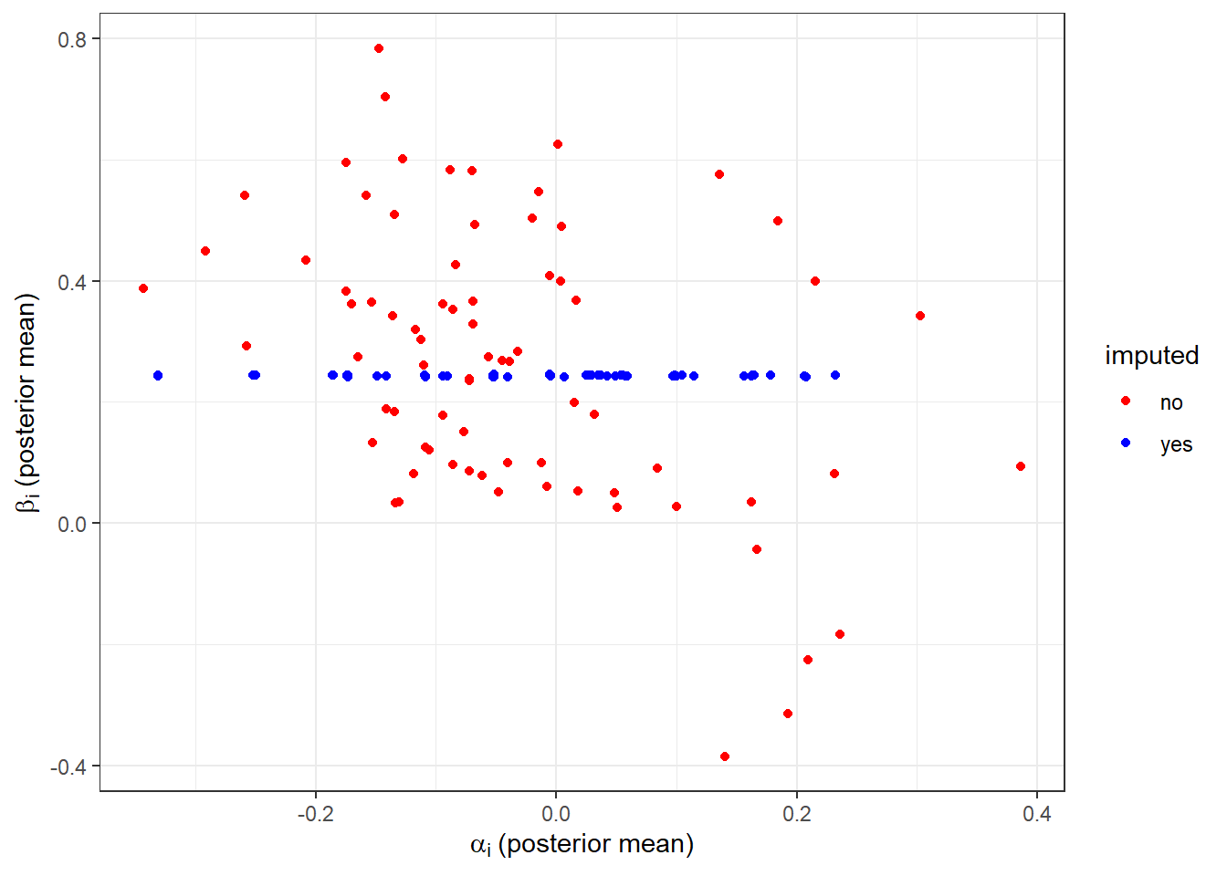
Figure 8.6: Posterior mean estimates of individual-level parameters using data with missing mixed and advantageous inequality participants. Model assumes identity correlation matrix (i.e. no correlation between the individual-level parameters).
Figure 8.6 shows the posterior mean estimates of \(\alpha_i\) and \(\beta_i\) for this model. This should be compared with Figure 8.3 (which includes the correlation matrix in the model). Here we can see that the imputed posterior means for \(\beta_i\) are basically the same number. They are in fact centered on the population mean parameter \(\mu_\beta\). Importantly, they do not vary with \(\alpha_i\) or \(\lambda_i\) becuase the model “knows” for sure that they don’t, and so any actual correlation between these parameters must be spurious (in the dogmatic eyes of the correlation-less model, at least).
8.5 Conclusion
Now we have a framework for filling in the gaps. Hopefully you can see the big picture in that all we really did was feed an appropriate hierarchical model the all data we had to work with, and then the hierarchical model filled in the gaps for us. In this application it was helpful to have some participants make decisions in all of the domains, because that helps pin down the correlation matrix. This correlation matrix is very important, because without it we would just be imputing marginal population means.
In other applications, there may be even more to condition on than the parameters themselves. For example, suppose an experiment also had a demographics survey. Allowing (say) the population means to vary by these demographics could provide even more information for the model to condition on. That is, if men and women are different in their mean \(\beta_i\)s, this information could also be conditioned on, but only if we estimate a model that allows for this at the population level.
For experiments that already exist, the ability to impute parameters that aren’t well-informed by the likelihood could be a useful tool for filling the gaps in the data. Additionally, for experiments in the design stage, there is perhaps work to be done in determining the optimal decisions to present to subjects in order to estimate the desired parameters. With imputation, it is not clear that it is optimal to present all participants with the same decisions, for example. Alternatively, suppose estimates of \(\alpha_i\) and \(\beta_i\) are something that we would like to include on the right-hand-side of a regression, where the dependent variable is behavior in another task.37 Perhaps due to time constraints, it may not be feasible to give the participants that do this second task all of the decisions in the Bruhin, Fehr, and Schunk (2019) dictator task. Instead, we could give them a subset of them (ideally, though, across all three domains), and rely on imputation to construct more reliable estimates using data from a second set of subjects who did make all of these choices (but did not participate in the second task).38
8.6 R code used for this chapter
library(tidyverse)
library(rstan)
options(mc.cores = parallel::detectCores())
rstan_options(auto_write = TRUE)

RERUN<-TRUE

set.seed(42)

d1<-(read.csv("Data/BFS2019_choices_exp1.csv")
     |> mutate(experiment=1)
)
d2<-(read.csv("Data/BFS2019_choices_exp2.csv")
     |> mutate(experiment=2)
)
D<-(rbind(d1,d2)
    # Just use the dictator game data
    |> filter(dg==1)
    |> mutate(
      self_alloc = ifelse(choice_x==1,self_x,self_y),
      other_alloc = ifelse(choice_x==1,other_x,other_y)
    )
) |>
  mutate(
    domain.x = ifelse(self_x>other_x,"adv","disadv"),
    domain.y = ifelse(self_y>other_y,"adv","disadv"),
    domain.overall = ifelse(domain.x == "adv" & domain.y == "adv","adv",
                            ifelse(domain.x == "disadv" & domain.y == "disadv","disadv",
                            "mixed")
                            )
  )

sid.list<-D |>
  select(sid) |>
  unique() |>
  mutate(
    i = 1:n()
  ) |>
  mutate(
    holdout = i<=(n()/2)
  )

D<-D |>
  full_join(sid.list,
        by = "sid"
            ) |>
  mutate(
    drop = (holdout & domain.overall == "mixed") | (holdout & domain.overall =="adv")
  )


model<-"Code/ImputingStuff/Hierarchical_BFS2019_correlated_onoff.stan" |>
  stan_model()

file<-"Code/ImputingStuff/00_run_leaveout_nocorr.csv"

if (!file.exists(file) | RERUN) {

  print("Estimating model with held-out data and no correlation matrix")

  d<- D |>
    filter(!drop)

  dStan<-list(
    n = dim(d)[1],
    self_x = d$self_x,
    other_x = d$other_x,
    self_y = d$self_y,
    other_y = d$other_y,
    choice_x = d$choice_x,

    id = d$i,
    nParticipants = max(d$i),

    prior_mu = rbind(c(0,0.39),
                     c(0,0.39),
                     c(-5.76,1)
    ),
    prior_tau = c(0.79,0.79,0.24),
    prior_LKJ = 2,

    UseCorr = 0

  )

  Fit<-model |>
    sampling(data=dStan,
             iter = 10000, chains=8,
             par = "z", include = FALSE,
             seed=42)

  summary(Fit)$summary |>
    data.frame() |>
    rownames_to_column(var = "par") |>
    write.csv(file)


}


file<-"Code/ImputingStuff/00_run_leaveout_corr.csv"

if (!file.exists(file) | RERUN) {

  print("Estimating model with held-out data and correlation matrix")

  d<- D |>
    filter(!drop)

  dStan<-list(
    n = dim(d)[1],
    self_x = d$self_x,
    other_x = d$other_x,
    self_y = d$self_y,
    other_y = d$other_y,
    choice_x = d$choice_x,

    id = d$i,
    nParticipants = max(d$i),

    prior_mu = rbind(c(0,0.39),
                     c(0,0.39),
                     c(-5.76,1)
    ),
    prior_tau = c(0.79,0.79,0.24),
    prior_LKJ = 2,

    UseCorr = 1

  )

  Fit<-model |>
    sampling(data=dStan,
             iter = 10000, chains=8,
             par = "z", include = FALSE,
             seed=42)

  summary(Fit)$summary |>
    data.frame() |>
    rownames_to_column(var = "par") |>
    write.csv(file)


}


file<-"Code/ImputingStuff/00_run_alldata.csv"

if (!file.exists(file) | RERUN) {

  print("Estimating model with all data")

  dStan<-list(
    n = dim(D)[1],
    self_x = D$self_x,
    other_x = D$other_x,
    self_y = D$self_y,
    other_y = D$other_y,
    choice_x = D$choice_x,

    id = D$i,
    nParticipants = max(D$i),

    prior_mu = rbind(c(0,0.39),
                     c(0,0.39),
                     c(-5.76,1)
    ),
    prior_tau = c(0.79,0.79,0.24),
    prior_LKJ = 2,

    UseCorr = 1

  )

  Fit<-model |>
    sampling(data=dStan,
             iter = 10000, chains=8,
             par = "z", include = FALSE,
             seed=42)

  summary(Fit)$summary |>
    data.frame() |>
    rownames_to_column(var = "par") |>
    write.csv(file)


}References
If you’ve been reading this book, you’re probably wondering why anyone wouldn’t put a correlation matrix into a hierarchical model, because I almost always put one into mine. I must say that until I started writing this chapter, I hadn’t thought much about why I was doing it, other than that I believe that parameters are correlated, and so I should estimate a model that permits this. In other words, I include correlation matrices in my models because … why not? More recently, I have walked this back a bit. For one thing, if you have informative enough data on all of the parameters, and you want to make inference about individuals (not the population), then there is a growing evidence showing that it really doesn’t matter practically, and a model without a covariance matrix will probably converge easier. But if you want to make statements about the population, then the correlation matrix itself might be interesting. Furthermore, if you are doing imputation, then it allows you to better condition your estimates on properties of the population. ↩︎
Here I color the dots based on imputation rather than \(\lambda_i\). The estimates of \(\lambda_i\) are of course still there, but just not shown in the plot. ↩︎
In fact there is also much less information about \(\alpha_i\) and \(\lambda_i\) because I threw out the mixed choices as well. Therefore if you squint enough you might see some more shrinkage for the blue dots horizontally as well. ↩︎
Really we should be jointly estimating this. Perhaps I will write another chapter on joint estimation of this form. ↩︎
This suggests that it could be useful to have a pool of well-collected data for a laboratory that is very informative of “standard” preference parameters (e.g. perhaps risk, time, other-regarding, and so on). These data could be used in multiple other experiments to help provide more precise estimates of the desired individual-level parameters. The trick here would be to make sure that these data are generated by a similar-enough subject pool that including them in the imputation is meaningful. Furthermore, as many experiments are moving online, and so the subject pools for (say) Prolific across different experiments may look very similar, this means that there may be great public good value in producing these datasets, and that these datasets should be well-cited if these methods are adopted, hint hint! ↩︎