24 Application: choice bracketing
This topic evokes some strong (mostly good) feelings for me, as I wrote my job market paper on it (James R. Bland 2019a). Choice bracketing is the idea that people might partition (or “bracket”) their decisions into more than one group. When I was on the job market, I would use the analogy of choosing what to eat and drink at a restaurant. The (unboundedly) rational economic agent who brackets broadly picks their favorite combination of food and drink. However this may be a difficult problem if the food and drink menus are large. Instead, the decision-maker might look only at the food menu and pick their favorite food, then look only at the drink menu and pick their favorite drink. This behavior is called narrow bracketing, and can lead to mistakes relative to the rational model because the decision-maker ignores that food and drink can be complements. For example, a narrowly bracketing decision-maker runs the risk at a restaurant of choosing red wine with fish, which is often regarded as a poor pairing.106
While we as humans usually pay some attention to the combinations of food and drink we are consuming, we may be more likely to narrowly bracket in other domains. One domain that has received a lot of attention in the experimental/behavioral economics and psychology literature is choice under risk (see for example Rabin and Weizsäcker (2009)). In this environment “mistakes” are sometimes easier to recognize because they can be identified by (e.g. first-order stochastically) dominated choices. However Ellis and Freeman (2024) argue that the existing literature typically provides evidence against broad bracketing, rather than in favor of narrow bracketing. That is, the broad bracketing model does not organize the data well, but the narrow bracketing model does not make any testable predictions for existing experiments. It is this experiment of Ellis and Freeman (2024) that I use as the example dataset in this chapter.
24.1 Data and model
For this application, I use data from the social preferences experiment in Ellis and Freeman (2024). In this experiment, made five decisions that involved allocating tokens to two other people. In decisions 2, 4, and 5, this was a simple convex budget set problem of allocating \(I\) tokens between person A and person B. Tokens were worth \(\$v_A\) to person A and \(\$v_B\) to person B. Figure 24.1 shows these decisions along with dicisions 1 and 3, which I will get to later. For decisions 2, 4, and 5, the red line shows the budget line, and the red dot shows the choice made by participant 6 in the experiment. Here we can see that in decision 4 participants faced a choice where tokens were equally valuable to person A and person B. In this instance participant 6 chose to split them equally. This is also approximately true for decision 2 (where tokens were also equally valuable). On the other hand in decision 5, tokens are worth more to person B than person A, and participant 6 chose to give all of the tokens to person B.
lookup<-rbind(
  # decision  part  I vA  vB
  c(1,1,10,1,1.20),
  c(1,2,16,1,1),
  c(2,1,14,2,2),
  c(3,1,10,1,1),
  c(3,2,10,1,1.20),
  c(4,1,16,1,1),
  c(5,1,10,1,1.20)
) |>
  data.frame()
colnames(lookup)<-c("decision","part","I","vA","vB")

D<-"Data/EF2024/SocialExperimentData.csv" |>
  read.csv()|>
  mutate(
    uid = paste(Location,Session,SubjectID) |> as.factor() |> as.numeric()
  ) |>
  pivot_longer(
    cols = R1A1.A:R5A1.B,
    names_to = "name",
    values_to = "allocation"
  )   |>
      mutate(
        decision = substr(name,2,2) |> as.integer(),
        part =  substr(name,4,4) |> as.integer(),
        player = substr(name,6,6)
  )|>
  filter(player=="A")|>
  full_join(lookup,by=c("decision","part")) |>
  mutate(
    decision = paste("decision",decision),
    part = paste("part",part)
  )


(
  ggplot(D |> filter(uid==6))
  +geom_segment(
    aes(
      x = I*vA,y=0,
      xend = 0, yend=I*vB,
      color=part
                ),linewidth=0.5)
  +facet_wrap(~decision)
  +geom_point(aes(x=allocation*vA,y=(I-allocation)*vB,color=part))
  +geom_vline(xintercept=0)+geom_hline(yintercept=0)
  +theme_minimal()
  +xlab("allocation to person A")+ylab("allocation to person B")
  +coord_fixed()
  +scale_color_manual(values = c("red", "blue"))
  +theme(legend.title = element_blank())
  #+geom_abline(slope=1,intercept=0,linetype="dashed")
)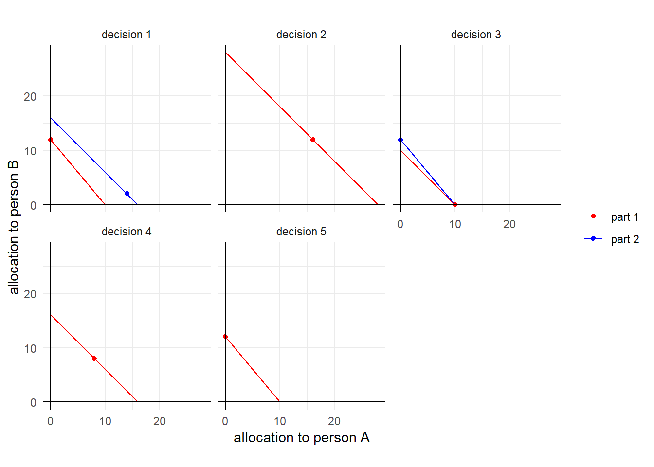
Figure 24.1: Choice data for participant 6, narrow framing.
Decisions 1 and 3 were slightly more complicated, in that the decision-maker faced two budget sets, with different endowments (\(I\)) and values to each person (\(v_A\),\(v_B\)). If one of these decisions was chosen for payment, then both parts of the decision would be added to person A and B’s earnings. For participant 6 in Figure 24.1 we can see that in decision 3, they allocated all of their part 2 tokens (blue) to person B, and all of their part 1 (red) tokens to person A.
To see how we might (qualitatively at least) distinguish between broad and narrow bracketing, I found it helpful to also look at the choice data for participant 1, which are shown in Figure 24.2. In particular, note in decision 3 that this participant chose close to the equal split for both parts of this decision. This could be rationalized under narrow bracketing by assuming that participant 1 likes payoff to be equal. However is cannot be rationalized under broad bracketing if we also assume that, all else held equal, participant 1 would like person A and B to get more money. This is becuase participant 1 could have allocated more part 1 tokens to A and more part 2 tokens to B, and both A and B could have received more earnings.
(
  ggplot(D |> filter(uid==1))
  +geom_segment(
    aes(
      x = I*vA,y=0,
      xend = 0, yend=I*vB,
      color=part
                ),linewidth=0.5)
  +facet_wrap(~decision)
  +geom_point(aes(x=allocation*vA,y=(I-allocation)*vB,color=part))
  +geom_vline(xintercept=0)+geom_hline(yintercept=0)
  +theme_minimal()
  +xlab("allocation to person A")+ylab("allocation to person B")
  +coord_fixed()
  +scale_color_manual(values = c("red", "blue"))
  +theme(legend.title = element_blank())
)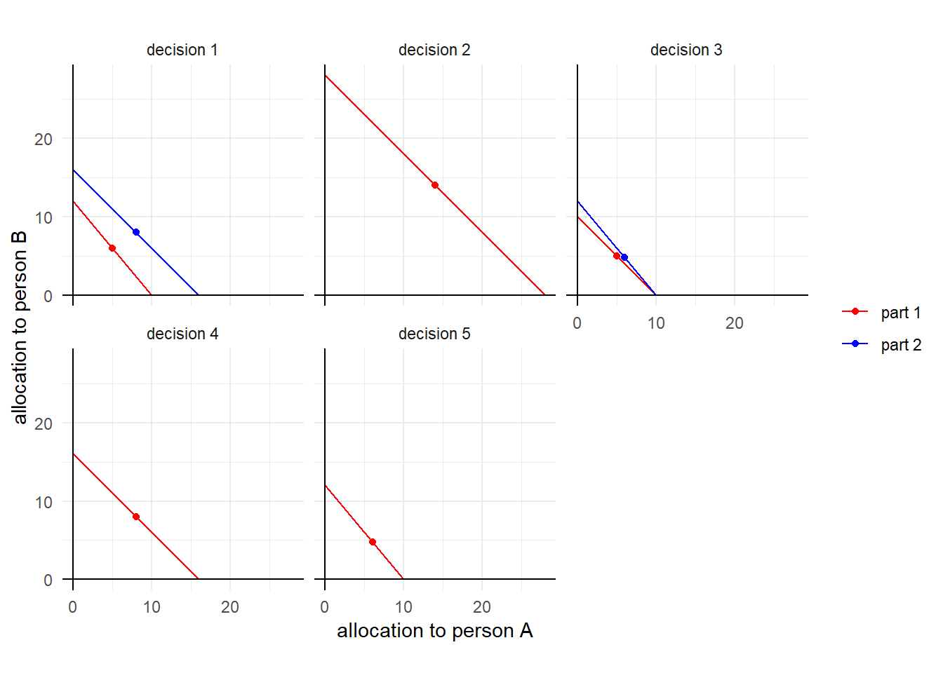
Figure 24.2: Choice data for participant 1, narrow framing.
In total, 102 participants made these five decisions. Choice sets were discretized to integer multiples of tokens, so in my analysis, I will assume logit choice over the discretized choice set.
So that’s the dataset, now we need a model for bracketing behavior. For this, I will use the \(\alpha\)-partial bracketing model (Barberis, Huang, and Thaler (2006), Barberis and Huang (2009), and Rabin and Weizsäcker (2009)). For this application, suppose that decision-makers have a utility function over earnings for person A and person B. which we denote \(u(x_A,x_B)\), where \(x_A\) and \(x_B\) are the monetary earnings of A and B, respectively. In a 1-part decision, the decision-maker’s utility-maximization problem is identical irrespective of how they bracket: \[ \begin{aligned} \max_{y_A+y_B\leq I_d} u(v_{A,d}y_A,\ v_{B,d}y_B) \end{aligned} \]
where \(I_d\) is token endowment in decision \(d\), and \(v_{A,d}\) and \(v_{B,d}\) are the values of these tokens to person A and person B, respectively (I am writing this as a continuous choice problem, but when I get to the econometric model this will of course be a discrete choice problem).
For the 2-part decisions, the decision-maker’s maximization problem if they broadly bracket is: \[ \begin{aligned} \max_{y^1_A+y^1_B\leq I^1_d,\ y^2_A+y^2_B\leq I^2_d} u(v^1_{A,d}y^1_A+v^2_{A,d}y^2_A,\ v^1_{B,d}y^1_B+v^2_{B,d}y^2_B) \end{aligned} \]
That is, a broadly-bracketing decision-maker adds up the payoffs that each recipient will get from each part of the decision. A narrowly-bracketing decision-maker, on the other hand, maximizes utility for each part of the decision separately. Therefore we can write their maximization problem as:
\[ \begin{aligned} \max_{y^1_A+y^1_B\leq I^1_d, \ y^2_A+y^2_B\leq I^2_d} u(v^1_{A,d}y^1_A,\ v^1_{B,d}y^1_B)+u(v^2_{A,d}y^2_A,\ v^2_{B,d}y^2_B) \end{aligned} \]
Note that, while I have written this as joint maximization over the sum of two utility functions, this problem can be solved in two parts because they are additively separable.
Now that we have a (deterministic) model of both narrow and broad bracketing, we can get to the partial bracketing part of the model. Here we just take a convex combination of the two utility functions: \[ \begin{aligned} \max_{y^1_A+y^1_B\leq I^1_d,\ y^2_A+y^2_B\leq I^2_d} \alpha \left( u(v^1_{A,d}y^1_A,\ v^1_{B,d}y^1_B)+u(v^2_{A,d}y^2_A,\ v^2_{B,d}y^2_B)\right) + (1-\alpha )u(v^1_{A,d}y^1_A+v^2_{A,d}y^2_A,\ v^1_{B,d}y^1_B+v^2_{B,d}y^2_B) \end{aligned} \]
where \(\alpha \in[0,1]\) is the extent of narrow bracketing, and \(\alpha=1\) (\(\alpha=0\)) corresponds to full narrow (broad) bracketing.
In order to make this an econometric model, we need to do two things. First, we need to assume a function form for \(u(\cdot,\cdot)\). I chose to go with a constant elasticity of substitution (CES) utility function here with equal weights on each of person A and B’s payoffs. Equal weights seems reasonable here because these were anonymous people in the lab, and so the decision-maker has no reason to value one of these people over another. Therefore, the functional form for the utility function will be: \[ u(x_A,x_B)=\left(x_A^\beta+x_B^\beta\right)^{\frac{1}{\beta}} \]
where \(\beta>0\) is another parameter to be estimated.
Finally, we need to add a probabilistic component to this deterministic model. Here I am going to use logit choice over the action space, and use \(\lambda>0\) as the choice precision parameter.
24.2 Representative agent and individual estimation
To begin with, I estimate a representative agent model, which I then also use to estimate on each participants’ data separately. These can both use the same Stan program: we just pass different data to it. In the Stan program below, you can see that I chose to hard-code the payoffs for each of the five decisions in Stan. While I usually try to avoid this kind of thing, my previous iteration of this was having to re-construct the choice set and payoffs for every decision. This is because the size of the choice set varies between decision. As such, the data passed to Stan is the allocation of tokens made to Person A (y1_1 and y1_2 for decision 1, and so on). In order to avoid a mess of code in the model block, I added two functions in the functions block. ll_1part computes the log-likelihood of a decision for decisions with only one part, and ll_2part does the same for decisions with two parts.
functions {

    real ll_1part(
      data vector payA, data vector payB,
      real beta, real lambda,
      data int y
    ) {

      int dim = dims(payA)[1];

      vector[dim] U = lambda*pow(pow(payA,beta)+pow(payB,beta),1.0/beta);


      return log_softmax(U)[y+1];

    }


    real ll_2part(
      data matrix payA1, data matrix payB1,
      data matrix payA2, data matrix payB2,
      real alpha, real beta, real lambda,
      data int y1, data int y2
    )  {

      int dim[2] = dims(payA1);

      // utility if DM brackets broadly
      matrix[dim[1],dim[2]] Ubroad = pow(
        pow(payA1+payA2,beta)+pow(payB1+payB2,beta)
      ,1.0/beta);

      // utility if DB brackets narrowly
      matrix[dim[1],dim[2]] Unarrow =
        pow(pow(payA1,beta)+pow(payB1,beta),1.0/beta)
        +pow(pow(payA2,beta)+pow(payB2,beta),1.0/beta)
        ;

      // partial bracketing utility
      matrix[dim[1],dim[2]] U = lambda*(alpha*Unarrow+(1.0-alpha)*Ubroad);

      return U[y1+1,y2+1]-log_sum_exp(U);

    }
}

data {
  int N;

  vector[2] prior_alpha;
  vector[2] prior_beta;
  vector[2] prior_lambda;

  // allocations to player A
  int y1_1[N];
  int y1_2[N];
  int y2[N];
  int y3_1[N];
  int y3_2[N];
  int y4[N];
  int y5[N];

}

transformed data {

  /* Here I am going to hard-code the experiment parameters and choice sets
  This is becuase each decision has different endowments (I),
  and so it saves a lot of matrix-creation on the fly in the
  model block
  */

  // decision 1, 2 parts --------------------
  int I1_1 = 10;
  int I1_2 = 16;
  real vA1_1 = 1;
  real vB1_1 = 1.2;
  real vA1_2 = 1;
  real vB1_2 = 1;

  matrix[I1_1+1,I1_2+1] X1_1 = rep_matrix(linspaced_vector(I1_1+1, 0, I1_1),I1_2+1);
  matrix[I1_1+1,I1_2+1] X1_2 = rep_matrix(linspaced_row_vector(I1_2+1, 0, I1_2),I1_1+1);

  matrix[I1_1+1,I1_2+1] payA1_1 = vA1_1*X1_1;
  matrix[I1_1+1,I1_2+1] payB1_1 = vB1_1*(I1_1-X1_1);
  matrix[I1_1+1,I1_2+1] payA1_2 = vA1_2*X1_2;
  matrix[I1_1+1,I1_2+1] payB1_2 = vB1_2*(I1_2-X1_2);

  // decision 2, 1 part -------------------
  int I2 = 14;
  real vA2 = 2;
  real vB2 = 2;

  vector[I2+1] X2 = linspaced_vector(I2+1, 0, I2);

  vector[I2+1] payA2 = vA2*X2;
  vector[I2+1] payB2 = vB2*(I2-X2);

  // decision 3, 2 parts --------------------
  int I3_1 = 10;
  int I3_2 = 10;
  real vA3_1 = 1;
  real vB3_1 = 1;
  real vA3_2 = 1;
  real vB3_2 = 1.2;

  matrix[I3_1+1,I3_2+1] X3_1 = rep_matrix(linspaced_vector(I3_1+1, 0, I3_1),I3_2+1);
  matrix[I3_1+1,I3_2+1] X3_2 = rep_matrix(linspaced_row_vector(I3_2+1, 0, I3_2),I3_1+1);

  matrix[I3_1+1,I3_2+1] payA3_1 = vA3_1*X3_1;
  matrix[I3_1+1,I3_2+1] payB3_1 = vB3_1*(I3_1-X3_1);
  matrix[I3_1+1,I3_2+1] payA3_2 = vA3_2*X3_2;
  matrix[I3_1+1,I3_2+1] payB3_2 = vB3_2*(I3_2-X3_2);

  // decision 4, 1 part -------------------
  int I4 = 16;
  real vA4 = 1;
  real vB4 = 1;

  vector[I4+1] X4 = linspaced_vector(I4+1, 0, I4);

  vector[I4+1] payA4 = vA4*X4;
  vector[I4+1] payB4 = vB4*(I4-X4);

   // decision 5, 1 part -------------------
  int I5 = 10;
  real vA5 = 1;
  real vB5 = 1.2;

  vector[I5+1] X5 = linspaced_vector(I5+1, 0, I5);

  vector[I5+1] payA5 = vA5*X5;
  vector[I5+1] payB5 = vB5*(I5-X5);


}


parameters {

  real<lower=0,upper=1> alpha;
  real<lower=0> beta;
  real<lower=0> lambda;

}


model {

  // priors---------------------------------------------------------------------

  alpha ~ beta(prior_alpha[1],prior_alpha[2]);
  beta ~ lognormal(prior_beta[1],prior_beta[2]);
  lambda ~ lognormal(prior_lambda[1],prior_lambda[2]);

  // likelihood ----------------------------------------------------------------

  for (ii in 1:N) {


    // decision 1, 2 parts
    target += ll_2part(
      payA1_1, payB1_1,
      payA1_2, payB1_2,
      alpha,beta,lambda,
      y1_1[ii],y1_2[ii]
    );


    // decision 2, 1 part
    target += ll_1part(
      payA2, payB2,
      beta, lambda,
      y2[ii]
    );

     // decision 3, 2 parts
    target += ll_2part(
      payA3_1, payB3_1,
      payA3_2, payB3_2,
      alpha,beta,lambda,
      y3_1[ii],y3_2[ii]
    );

    // decision 4, 1 part
    target += ll_1part(
      payA4, payB4,
      beta, lambda,
      y4[ii]
    );

    // decision 5, 1 part
    target += ll_1part(
      payA5, payB5,
      beta, lambda,
      y5[ii]
    );


  }


}
Table 24.1 summarizes the posterior distribution of the representative agent model. Of primary interest here is the estimate for \(\alpha\), which is fairly precisely estimated to be about 20%. That is, the representative agent partially brackets, but their behavior is closer to broad bracketing than narrow bracketing.
"Code/EF2024/social_repagent.csv" |>
  read.csv() |>
  dplyr::select(-X) |>
  kbl(digits=3,caption = "Summary of posterior distribution from the representative agent model.") |>
  kable_classic(full_width=FALSE) |>
add_header_above(c("","","","","percentiles"=5,"",""))|
percentiles
|
||||||||||
|---|---|---|---|---|---|---|---|---|---|---|
| par | mean | se_mean | sd | X2.5. | X25. | X50. | X75. | X97.5. | n_eff | Rhat |
| alpha | 0.208 | 0.001 | 0.033 | 0.148 | 0.185 | 0.206 | 0.228 | 0.274 | 3830.117 | 1.002 |
| beta | 0.515 | 0.001 | 0.036 | 0.440 | 0.492 | 0.516 | 0.539 | 0.579 | 2897.681 | 1.005 |
| lambda | 0.729 | 0.002 | 0.120 | 0.499 | 0.645 | 0.727 | 0.808 | 0.969 | 2970.372 | 1.005 |
| lp__ | -1514.550 | 0.022 | 1.253 | -1517.772 | -1515.102 | -1514.220 | -1513.636 | -1513.127 | 3228.642 | 1.002 |
Next, I loop through each participant individually. Figure 24.3 shows the empirical cumulative density function of the posterior mean estimates of \(\alpha\). Here we can see that the majority of participants narrowly bracket to an extent of at least 50%, but no participant is close to fully narrowly bracketing their decisions. There are also a few participants with \(\alpha\) very close to zero, indicating that they broadly bracket their decisions.107
d<-"Code/EF2024/social_individual.csv" |>
  read.csv() |>
  filter(par=="alpha") |>
  mutate(
    cumul = rank(mean)/n()-0.5/n()
  )

(
  ggplot(d,aes(x=mean))
  +stat_ecdf()
  +theme_bw()
  +geom_errorbar(aes(xmin = X25.,xmax = X75., y=cumul),alpha=0.5,color="red")
  +xlim(c(0,1))
  +xlab(expression(alpha~"(extent of narrow bracketing)"))
  +ylab("cumulative density of posterior mean")
)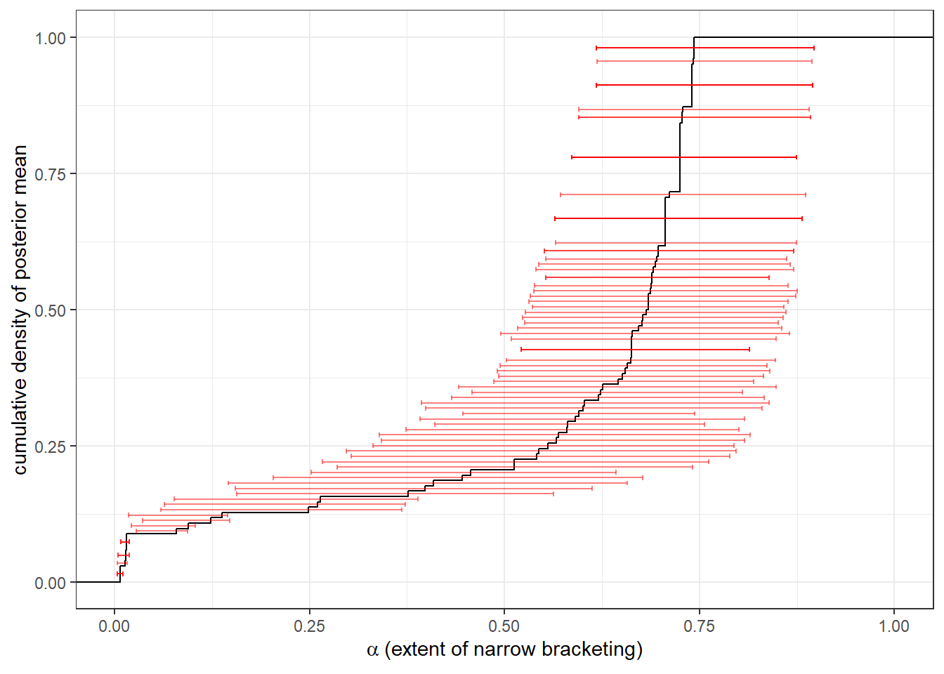
Figure 24.3: Estimates of extent of narrow bracketing at the individual level. Black line shows the empirical cumulative distribution function of the posterior mean. Red error bars show 50% Bayesian credible regions (25th-75th percentile)
While we might not be too interested in the other parameters in the model, it doesn’t hurt to take a quick look at them and make sure that there are no surprises. While I don’t have much intuition about what a reasonable value for \(\lambda\) is,108 a priori it seems like we should mostly be estimating \(0<\beta<1\). \(0<\beta\) will always be true because I encoded it into the prior, but \(\beta<1\) is particularly important becuase it indicates that the utility function is quasiconcave. For us, this means that our participants have convex preferences over person A and B’s earnings, which seems reasonable here. Let’s check it in Figure 24.4:
d<-"Code/EF2024/social_individual.csv" |>
  read.csv() |>
  filter(par=="beta")  |>
  mutate(
    cumul = rank(mean)/n()-0.5/n()
  )

(
  ggplot(d,aes(x=mean))
  +stat_ecdf()
  +theme_bw()
  +geom_errorbar(aes(xmin = X25.,xmax = X75., y=cumul),alpha=0.5,color="red")
  #+xlim(c(0,1))
  +xlab(expression(beta))
  +ylab("cumulative density of posterior mean")
)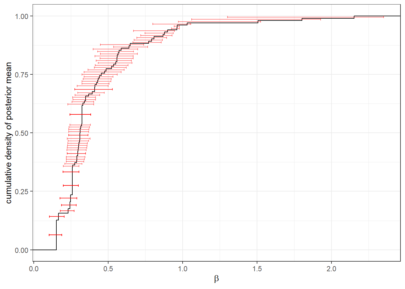
Figure 24.4: Estimates of \(\beta\) at the individual level. Black line shows the empirical cumulative distribution function of the posterior mean. Red error bars show 50% Bayesian credible regions (25th-75th percentile)
\(\beta<1\) for the vast majority of participants, good!
Before moving on to the hierarchical model, I want to stress an important thing that we would have missed if we only estimated the representative agent model. Recall that in the representative agent model we estimated \(\alpha\approx0.2\). However a quick-and-dirty sample mean of the posterior means from the individual-level estimations yields:
## [1] 0.4122716So our conclusions about bracketing would be vastly different depending on which of these summary statistics we believed! The representative agent model would have us believe that narrow bracketing is only a little bit important, and that decisions are closer to broad bracketing. On the other hand, the individual-level estimation suggests that most people bracket substantially closer to narrow than broad.
24.3 Hierarchical model
Here is the Stan program I wrote to estimate the hierarchical model. It of course looks very similar to the representative agent model except for the bits where the individual-level parameters go in. This is why I always want you to write and estimate the representative agent model first, even if you’re not going to use it: it is a very important stepping stone in getting to the richer hierarchical model, and will probably help you iron out a lot of the problems that are specific to your application (for this one, it was working out an efficient way to hard-code the experiment parameters).
functions {

    real ll_1part(
      data vector payA, data vector payB,
      real beta, real lambda,
      data int y
    ) {

      int dim = dims(payA)[1];

      vector[dim] U = lambda*pow(pow(payA,beta)+pow(payB,beta),1.0/beta);


      return log_softmax(U)[y+1];

    }


    real ll_2part(
      data matrix payA1, data matrix payB1,
      data matrix payA2, data matrix payB2,
      real alpha, real beta, real lambda,
      data int y1, data int y2
    )  {

      int dim[2] = dims(payA1);

      // utility if DM brackets broadly
      matrix[dim[1],dim[2]] Ubroad = pow(
        pow(payA1+payA2,beta)+pow(payB1+payB2,beta)
      ,1.0/beta);

      // utility if DB brackets narrowly
      matrix[dim[1],dim[2]] Unarrow =
        pow(pow(payA1,beta)+pow(payB1,beta),1.0/beta)
        +pow(pow(payA2,beta)+pow(payB2,beta),1.0/beta)
        ;

      // partial bracketing utility
      matrix[dim[1],dim[2]] U = lambda*(alpha*Unarrow+(1.0-alpha)*Ubroad);

      return U[y1+1,y2+1]-log_sum_exp(U);

    }
}

data {
  int N; // number of participants

  vector[3] prior_MU[2];
  vector[3] prior_TAU;
  real prior_Omega;

  // allocations to player A
  int y1_1[N];
  int y1_2[N];
  int y2[N];
  int y3_1[N];
  int y3_2[N];
  int y4[N];
  int y5[N];

}

transformed data {

  /* Here I am going to hard-code the experiment parameters and choice sets
  This is becuase each decision has different endowments (I),
  and so it saves a lot of matrix-creation on the fly in the
  model block
  */

  // decision 1, 2 parts --------------------
  int I1_1 = 10;
  int I1_2 = 16;
  real vA1_1 = 1;
  real vB1_1 = 1.2;
  real vA1_2 = 1;
  real vB1_2 = 1;

  matrix[I1_1+1,I1_2+1] X1_1 = rep_matrix(linspaced_vector(I1_1+1, 0, I1_1),I1_2+1);
  matrix[I1_1+1,I1_2+1] X1_2 = rep_matrix(linspaced_row_vector(I1_2+1, 0, I1_2),I1_1+1);

  matrix[I1_1+1,I1_2+1] payA1_1 = vA1_1*X1_1;
  matrix[I1_1+1,I1_2+1] payB1_1 = vB1_1*(I1_1-X1_1);
  matrix[I1_1+1,I1_2+1] payA1_2 = vA1_2*X1_2;
  matrix[I1_1+1,I1_2+1] payB1_2 = vB1_2*(I1_2-X1_2);

  // decision 2, 1 part -------------------
  int I2 = 14;
  real vA2 = 2;
  real vB2 = 2;

  vector[I2+1] X2 = linspaced_vector(I2+1, 0, I2);

  vector[I2+1] payA2 = vA2*X2;
  vector[I2+1] payB2 = vB2*(I2-X2);

  // decision 3, 2 parts --------------------
  int I3_1 = 10;
  int I3_2 = 10;
  real vA3_1 = 1;
  real vB3_1 = 1;
  real vA3_2 = 1;
  real vB3_2 = 1.2;

  matrix[I3_1+1,I3_2+1] X3_1 = rep_matrix(linspaced_vector(I3_1+1, 0, I3_1),I3_2+1);
  matrix[I3_1+1,I3_2+1] X3_2 = rep_matrix(linspaced_row_vector(I3_2+1, 0, I3_2),I3_1+1);

  matrix[I3_1+1,I3_2+1] payA3_1 = vA3_1*X3_1;
  matrix[I3_1+1,I3_2+1] payB3_1 = vB3_1*(I3_1-X3_1);
  matrix[I3_1+1,I3_2+1] payA3_2 = vA3_2*X3_2;
  matrix[I3_1+1,I3_2+1] payB3_2 = vB3_2*(I3_2-X3_2);

  // decision 4, 1 part -------------------
  int I4 = 16;
  real vA4 = 1;
  real vB4 = 1;

  vector[I4+1] X4 = linspaced_vector(I4+1, 0, I4);

  vector[I4+1] payA4 = vA4*X4;
  vector[I4+1] payB4 = vB4*(I4-X4);

   // decision 5, 1 part -------------------
  int I5 = 10;
  real vA5 = 1;
  real vB5 = 1.2;

  vector[I5+1] X5 = linspaced_vector(I5+1, 0, I5);

  vector[I5+1] payA5 = vA5*X5;
  vector[I5+1] payB5 = vB5*(I5-X5);


}


parameters {

  vector[3] MU;
  vector<lower=0>[3] TAU;
  cholesky_factor_corr[3] L_Omega;

  matrix[3,N] z;

}

transformed parameters {

  vector[N] alpha;
  vector[N] beta;
  vector[N] lambda;

  {
    matrix[3,N] theta = rep_matrix(MU,N)
                    //+diag_matrix(TAU)*z;
                    +diag_pre_multiply(TAU,L_Omega)*z;

    alpha = Phi_approx(theta[1,]');
    beta = exp(theta[2,]');
    lambda = exp(theta[3,]');

  }

}


model {

  // hierarchical structure with noncentered parameterization ------------------
  to_vector(z) ~ std_normal();

  // priors---------------------------------------------------------------------
  MU ~ normal(prior_MU[1],prior_MU[2]);
  TAU ~ cauchy(0.0,prior_TAU);
  L_Omega ~ lkj_corr_cholesky(prior_Omega);


  // likelihood ----------------------------------------------------------------

  for (ii in 1:N) {

    real a = alpha[ii];
    real b = beta[ii];
    real l = lambda[ii];

    // decision 1, 2 parts
    target += ll_2part(
      payA1_1, payB1_1,
      payA1_2, payB1_2,
      a,b,l,
      y1_1[ii],y1_2[ii]
    );


    // decision 2, 1 part
    target += ll_1part(
      payA2, payB2,
      b,l,
      y2[ii]
    );

     // decision 3, 2 parts
    target += ll_2part(
      payA3_1, payB3_1,
      payA3_2, payB3_2,
      a,b,l,
      y3_1[ii],y3_2[ii]
    );

    // decision 4, 1 part
    target += ll_1part(
      payA4, payB4,
      b,l,
      y4[ii]
    );

    // decision 5, 1 part
    target += ll_1part(
      payA5, payB5,
      b,l,
      y5[ii]
    );


  }


}
Figure 24.5 shows the shrinkage estimates for \(\alpha\) from the hierarchical model. (These have the same interpretation as the individual-level estimates in Figure 24.3). What struck me as surprising here (and I really should have seen it when I looked at the individual-level estimates in Figure @ref(fig:EF2024-individualecdf,)) was the bi-modality of a distribution. In an ecdf you can see the modes of a distribution as very steep parts. There appears to be one at about \(\alpha=0.4\), and another at \(\alpha=0.75\). This may pose a problem for the hierarchical model, which (and I’m waving my hands a lot here) is really hoping for a uni-modal distribution, or even better yet, a continuous normal distribution (of the transformed variable). This can be addressed by selecting a more flexible distribution, but I will leave this for another day.
d<-"Code/EF2024/social_hierarchical.csv" |>
  read.csv() |>
  filter(grepl("alpha",par)) |>
  mutate(
    cumul = rank(mean)/n()-0.5/n()
  )

(
  ggplot(d,aes(x=mean))
  +stat_ecdf()
  +theme_bw()
  +geom_errorbar(aes(xmin = X25.,xmax = X75., y=cumul),alpha=0.5,color="red")
  +xlim(c(0,1))
  +xlab(expression(alpha~"(extent of narrow bracketing)"))
  +ylab("cumulative density of posterior mean")
)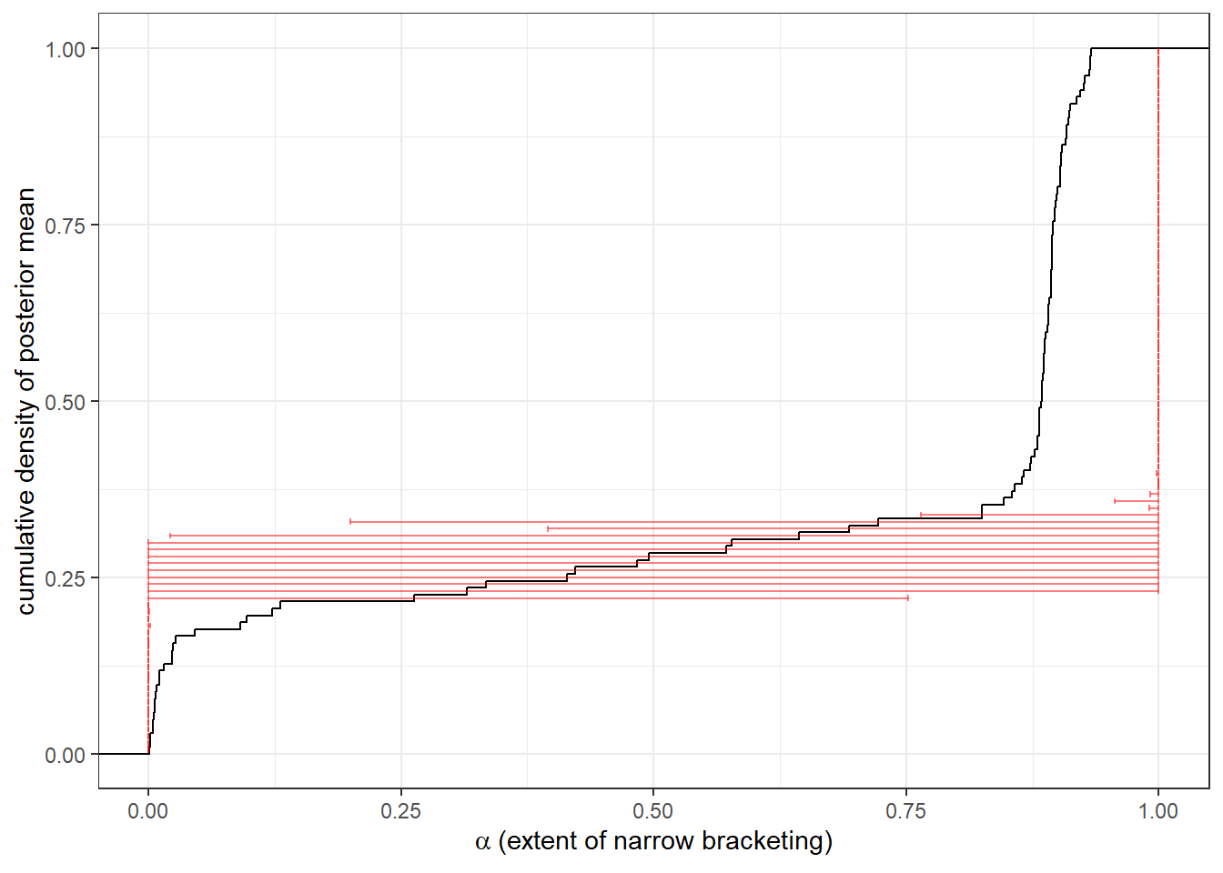
Figure 24.5: Shrinkage estimates of extent of narrow bracketing at the individual level from the hierarchical model. Black line shows the empirical cumulative distribution function of the posterior mean. Red error bars show 50% Bayesian credible regions (25th-75th percentile)
24.4 A mixture model
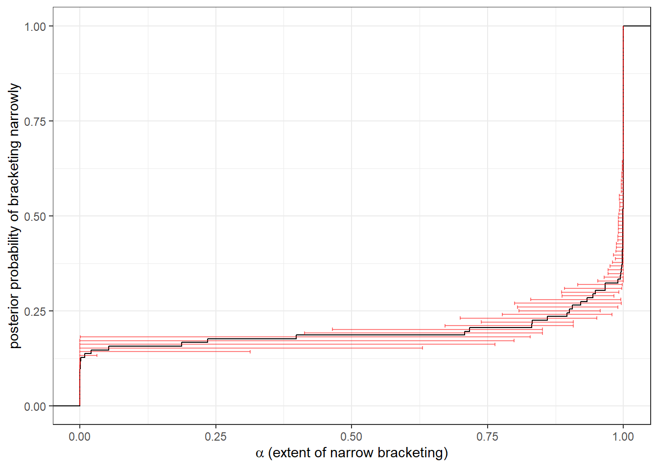
One thing that I was worried about while doing the above work was that there were only five decisions per participant. Furthermore only two of these decisions had two parts, and so it was really only these decisions that provided us with information about \(\alpha\), the extent of narrow bracketing.109 This is certainly reflected in the large credible regions for \(\alpha\) for the individual-level estimation (recall that these were only 50% credible regions), and so we are not estimating \(\alpha\) particularly precisely. Instead of assuming the partial bracketing model, we could simplify things by instead assuming that participants either fully narrowly bracketed or fully broadly bracketed. That is, we have a 2-type (discrete) mixture model. At the individual level, this turns the problem from an estimation (of \(\alpha\)) problem to a classification (into \(\alpha=0\) or \(\alpha=1\)) problem. Our model will now tell us the fraction of narrow bracketers in the population, and we will be able to assign a posterior probability to each participant that they are a narrow bracketer.
Here is the Stan program I wrote to estimate this mixture model. Importantly, I am preserving the hierarchical structure for the parameters \(\beta\) and \(\lambda\), which if we are just interested in bracketing behavior, could be considered nuisance parameters for this inferential goal.110 Hence, our model will be in some sense robust to participant-level heterogeneity in these parameters. Note that I have moved a lot of the calculations into the transofrmed parameters block so I can use the ll variable into both the model (to increment the log-posterior) and generated quantities (to calculate posterior type probabilities) blocks.
functions {

    real ll_1part(
      data vector payA, data vector payB,
      real beta, real lambda,
      data int y
    ) {

      int dim = dims(payA)[1];

      vector[dim] U = lambda*pow(pow(payA,beta)+pow(payB,beta),1.0/beta);


      return log_softmax(U)[y+1];

    }


    real ll_2part(
      data matrix payA1, data matrix payB1,
      data matrix payA2, data matrix payB2,
      real alpha, real beta, real lambda,
      data int y1, data int y2
    )  {

      int dim[2] = dims(payA1);

      // utility if DM brackets broadly
      matrix[dim[1],dim[2]] Ubroad = pow(
        pow(payA1+payA2,beta)+pow(payB1+payB2,beta)
      ,1.0/beta);

      // utility if DB brackets narrowly
      matrix[dim[1],dim[2]] Unarrow =
        pow(pow(payA1,beta)+pow(payB1,beta),1.0/beta)
        +pow(pow(payA2,beta)+pow(payB2,beta),1.0/beta)
        ;

      // partial bracketing utility
      matrix[dim[1],dim[2]] U = lambda*(alpha*Unarrow+(1.0-alpha)*Ubroad);

      return U[y1+1,y2+1]-log_sum_exp(U);

    }
}

data {
  int N; // number of participants

  vector[2] prior_MU[2];
  vector[2] prior_TAU;
  real prior_Omega;
  vector<lower=0.0>[2] prior_mix;

  // allocations to player A
  int y1_1[N];
  int y1_2[N];
  int y2[N];
  int y3_1[N];
  int y3_2[N];
  int y4[N];
  int y5[N];

}

transformed data {

  /* Here I am going to hard-code the experiment parameters and choice sets
  This is becuase each decision has different endowments (I),
  and so it saves a lot of matrix-creation on the fly in the
  model block
  */

  // decision 1, 2 parts --------------------
  int I1_1 = 10;
  int I1_2 = 16;
  real vA1_1 = 1;
  real vB1_1 = 1.2;
  real vA1_2 = 1;
  real vB1_2 = 1;

  matrix[I1_1+1,I1_2+1] X1_1 = rep_matrix(linspaced_vector(I1_1+1, 0, I1_1),I1_2+1);
  matrix[I1_1+1,I1_2+1] X1_2 = rep_matrix(linspaced_row_vector(I1_2+1, 0, I1_2),I1_1+1);

  matrix[I1_1+1,I1_2+1] payA1_1 = vA1_1*X1_1;
  matrix[I1_1+1,I1_2+1] payB1_1 = vB1_1*(I1_1-X1_1);
  matrix[I1_1+1,I1_2+1] payA1_2 = vA1_2*X1_2;
  matrix[I1_1+1,I1_2+1] payB1_2 = vB1_2*(I1_2-X1_2);

  // decision 2, 1 part -------------------
  int I2 = 14;
  real vA2 = 2;
  real vB2 = 2;

  vector[I2+1] X2 = linspaced_vector(I2+1, 0, I2);

  vector[I2+1] payA2 = vA2*X2;
  vector[I2+1] payB2 = vB2*(I2-X2);

  // decision 3, 2 parts --------------------
  int I3_1 = 10;
  int I3_2 = 10;
  real vA3_1 = 1;
  real vB3_1 = 1;
  real vA3_2 = 1;
  real vB3_2 = 1.2;

  matrix[I3_1+1,I3_2+1] X3_1 = rep_matrix(linspaced_vector(I3_1+1, 0, I3_1),I3_2+1);
  matrix[I3_1+1,I3_2+1] X3_2 = rep_matrix(linspaced_row_vector(I3_2+1, 0, I3_2),I3_1+1);

  matrix[I3_1+1,I3_2+1] payA3_1 = vA3_1*X3_1;
  matrix[I3_1+1,I3_2+1] payB3_1 = vB3_1*(I3_1-X3_1);
  matrix[I3_1+1,I3_2+1] payA3_2 = vA3_2*X3_2;
  matrix[I3_1+1,I3_2+1] payB3_2 = vB3_2*(I3_2-X3_2);

  // decision 4, 1 part -------------------
  int I4 = 16;
  real vA4 = 1;
  real vB4 = 1;

  vector[I4+1] X4 = linspaced_vector(I4+1, 0, I4);

  vector[I4+1] payA4 = vA4*X4;
  vector[I4+1] payB4 = vB4*(I4-X4);

   // decision 5, 1 part -------------------
  int I5 = 10;
  real vA5 = 1;
  real vB5 = 1.2;

  vector[I5+1] X5 = linspaced_vector(I5+1, 0, I5);

  vector[I5+1] payA5 = vA5*X5;
  vector[I5+1] payB5 = vB5*(I5-X5);


}


parameters {

  vector[2] MU;
  vector<lower=0>[2] TAU;
  cholesky_factor_corr[2] L_Omega;
  real<lower=0,upper=1> mix_narrow;

  matrix[2,N] z;

}

transformed parameters {

  vector[N] beta;
  vector[N] lambda;

  matrix[N,2] ll;

  {
    matrix[2,N] theta = rep_matrix(MU,N)
                    //+diag_matrix(TAU)*z;
                    +diag_pre_multiply(TAU,L_Omega)*z;

    beta = exp(theta[1,]');
    lambda = exp(theta[2,]');


    // likelihood computation ----------------------------------------------------------------

  for (ii in 1:N) {

    row_vector[2] ll_i = [log(mix_narrow),log(1.0-mix_narrow)];

    real b = beta[ii];
    real l = lambda[ii];

    // decision 1, 2 parts,
    //narrow
    ll_i[1] += ll_2part(
      payA1_1, payB1_1,
      payA1_2, payB1_2,
      1.0,b,l,
      y1_1[ii],y1_2[ii]
    );
    // broad
    ll_i[2] += ll_2part(
      payA1_1, payB1_1,
      payA1_2, payB1_2,
      0.0,b,l,
      y1_1[ii],y1_2[ii]
    );

    // decision 2, 1 part
    ll_i += ll_1part(
      payA2, payB2,
      b,l,
      y2[ii]
    );

     // decision 3, 2 parts
     // narrow
     ll_i[1] += ll_2part(
      payA3_1, payB3_1,
      payA3_2, payB3_2,
      1.0,b,l,
      y3_1[ii],y3_2[ii]
    );
    // broad
     ll_i[2] += ll_2part(
      payA3_1, payB3_1,
      payA3_2, payB3_2,
      0.0,b,l,
      y3_1[ii],y3_2[ii]
    );

    // decision 4, 1 part
    ll_i += ll_1part(
      payA4, payB4,
      b,l,
      y4[ii]
    );

    // decision 5, 1 part
    ll_i += ll_1part(
      payA5, payB5,
      b,l,
      y5[ii]
    );

    ll[ii,] = ll_i;
  }

  }

}


model {

  // hierarchical structure with noncentered parameterization ------------------
  to_vector(z) ~ std_normal();

  // priors---------------------------------------------------------------------
  MU ~ normal(prior_MU[1],prior_MU[2]);
  TAU ~ cauchy(0.0,prior_TAU);
  L_Omega ~ lkj_corr_cholesky(prior_Omega);
  mix_narrow ~ beta(prior_mix[1],prior_mix[2]);


  for (ii in 1:N) {
    target+= log_sum_exp(ll[ii,]);
  }

}

generated quantities {

  vector[N] postprob_narrow;
  for (ii in 1:N) {
    postprob_narrow[ii] = softmax(ll[ii,]')[1];
  }

}d<-"Code/EF2024/social_mixture.csv" |>
read.csv() |>
filter(grepl("postprob",par))|>
mutate(
cumul = rank(mean)/n()-0.5/n()
)
(
ggplot(d,aes(x=mean))
+stat_ecdf()
+theme_bw()
+geom_errorbar(aes(xmin = X2.5.,xmax = X97.5., y=cumul),alpha=0.5,color="red")
+xlim(c(0,1))
+xlab(expression(alpha~"(extent of narrow bracketing)"))
+ylab("posterior probability of bracketing narrowly")
)
24.5 What do we get out of the structural models, and what could we miss?
I have analyzed these data in a really different way to Ellis and Freeman (2024). There is no “Bayesian alternative to a maximum likelihood implementation” for me to do here like I can do for (say) strategy frequency estimation or structurally estimating risk preferences. Ellis and Freeman (2024) use nonparametric measures of mistakes to classify participants based on the number of mistakes they make relative to (say) Weak Axiom of Revealed Preference (WARP) predictions. Loosely speaking, this kind of analysis can put participants into three bins: (i) narrow bracketing, (ii) broad bracketing, and (iii) something else. This “something else” bin is really important, because it could be that participants are doing something other than narrowly or broadly bracketing. Ignoring this bin means that we will mis-classify these “something else” participants into one of the bracketing bins. This mis-classification may not be random, and so the resulting fractions may over- or under-state the prevalence of each bracketing behavior in the sample.
On the other hand, my approach forces every participant to be a partial bracketer (with different extents of bracketing, \(\alpha\)), or in the case of the mixture model, forces everybody to be either a broad or narrow bracketer. Out of this we get an easily interpretable measure of bracketing behavior for each participant, but we cannot say anything about the “something else”. This is not to say that we couldn’t also include something else in the structural model, but it would have to be a specific “something else” in the form of another parametric model.
References
While I was on the job market, after giving this analogy, a former professor of mine interrupted my talk to very loudly proclaim: “James, red wine is never a mistake!” Another former professor later volunteered that while he was on the job market, he ended up ordering fish and Coca-Cola, which for him turned out to be a particularly bad pairing.↩︎
The model would never estimate that a participant either fully brackets broadly (\(\alpha=0\)) or fully brackets narrowly (\(\alpha =1\)). This is becuase prior weight is placed on the interior of the unit interval.↩︎
Read: “Today I am too lazy to make a few plots to help my intuition here.”↩︎
It is not that the other three decisions provided us with nothing. They help pin down \(\beta\) and \(\lambda\) so that less uncertainty in these variables propogates into uncertainty in \(\alpha\).↩︎
If instead we wanted to (say) assign a welfare measure to narrow bracketing (e.g. “how much utility does someone give up by bracketing narrowly?”) then these might not be nuisance parameters. See James R. Bland (2019a) and James R. Bland (2019b) for examples of this.↩︎