9 More filling in the blanks: data augmentation
Sometimes in Bayesian computation, we can benefit from a technique called data augmentation. Here, we recognize that we can represent our model as a function of some latent variables, and estimate these latent variables alongside the parameters of interest. In fact, we have been doing this already in our hierarchical models. Here the latent variables are the individual-level parameters (which I usually denote \(\{\theta_i\}_{i=1}^N\) unless there is any other context for them), and we estimate these alongside the population-level parameters of our model. If we are estimating a hierarchical model, then we might actually be interested in these parameters. After all, in our structural models they often represent the parameters of interest if we want to make inference about the individual. On the other hand, there may be other situations where we can find a representation of our data-generating process that includes latent “nuisance” parameters that we don’t directly care about, but aid in the estimation process.
9.1 Example 1: two ways to estimate a probit model
To fix ideas, consider estimating a simple probit model, which we can write as:
\[ \begin{aligned} y&\sim \mathrm{Bernoulli}\Phi(X\beta) & \quad \text{(likelihood)}\\ \beta_k &\sim N(m_k,s_k^2)&\quad\text{(prior)} \end{aligned} \]
where \(\Phi(\cdot)\) is the standard normal cdf. While I have been trained in the classic Bayesian arts,39 this is how I mostly think of a probit. For me, this is because it directly encodes the model’s prediction in the likelihood: the probability of a success given \(X_i\) is \(\Phi(X_i\beta)\). Furthermore, this is how I would code it up in Stan:
data {
  int<lower=0> N; // number of observations
  int<lower=0> k; // number of explanatory variables
  matrix[N,k] X; // explanatory variables
  array[N] int<lower=0,upper=1> y; // binary outcome

  array[k] vector[2] prior_beta;
}


parameters {

  vector[k] beta;

}


model {

  // likelihood

  y ~ bernoulli(Phi(X*beta));

  // prior
  for (kk in 1:k) {
    beta[kk] ~ normal(prior_beta[kk][1],prior_beta[kk][2]);
  }

}
However not so long ago, this representation was much less efficient to sample from than the following latent variable representation:
\[ \begin{aligned} y^*&\sim N(X\beta,1^2)&\quad \text{(latent process)}\\ y_i&=\begin{cases} 1&\text{if } y_i^*\geq 0\\ 0&\text{if } y_i^*<0 \end{cases} & \quad \text{(observed outcome variable)}\\ \beta_k &\sim N(m_k,s_k^2)&\quad\text{(prior)} \end{aligned} \]
Here, we recognize that we can represent the observed data-generating process by a latent variable \(y^*\) which is greater than zero if we observe a one, and less than zero if we observe a zero. In essence, our binary outcome variable tells us the sign of \(y^*\). The reason this representation was really useful is because
- Conditional on the data and \(\beta\), it is really easy to sample from the posterior distribution of \(y^*\) because it is a truncated normal.
- Conditional on \(y^*\), the problem of sampling from the posterior distribution of \(\beta\) is exactly the same as if \(y^*\) were observed. Since this is just a linear regression model (with standard normal errors), this is really easy too.
As such, this fits nicely into a Gibbs sampler. We can estimate this version of the probit model in Stan as follows:
data {
  int<lower=0> N; // number of observations
  int<lower=0> k; // number of explanatory variables
  matrix[N,k] X; // explanatory variables
  array[N] int<lower=0,upper=1> y; // binary outcome

  array[k] vector[2] prior_beta;

  // pass a really large and positive number in here
  real Inf;
}

transformed data {

  // lower and upper bounds for the latent variables
  vector[N] y_lb;
  vector[N] y_ub;

  for (ii in 1:N) {

    y_lb[ii] = y[ii]==1 ? 0.0 : -Inf;
    y_ub[ii] = y[ii]==1 ? Inf : 0.0;

  }

}


parameters {

  vector[k] beta;

  // augmented data
  vector<lower=y_lb,upper=y_ub>[N] ystar;

}


model {

  // likelihood

  ystar ~ normal(X*beta, 1.0);

  // prior
  for (kk in 1:k) {
    beta[kk] ~ normal(prior_beta[kk][1],prior_beta[kk][2]);
  }

}
However since Stan doesn’t do Gibbs sampling, it will probably just give you the same results as the first implementation (without the latent variable), but with a longer runtime and a bigger RAM and CPU requirement. This isn’t to say that data augmentation is useless with modern Bayesian computing. Rather, the useful applications of data-augmentation just look a little different.
9.2 Example 2: accounting for rounded answers
In many economic experiments, we ask participants to choose a number between zero and one hundred. In these situations, participants might round their answers to the nearest (say) five or ten, and sometimes experiment programs might force the participant to round to the nearest one. As such, participants’ data cannot be interpreted as point-valued, and it is probably better to treat them as interval-valued. To illustrate this, consider Figure 9.1, which shows the distribution of the last digit of percentage reported beliefs in the four treatments of Holt and Smith (2016). Here we can see that the modal last digit is zero, indicating that a participant’s answer was a multiple of ten percentage points, and the next most common answer was a multiple of five percentage points. Here I distinguish between boundary decisions (red, i.e. reporting 100% or 0%) and interior decisions (gray, everything else).
D<-"Code/HS2016/cleaneddata.csv" |>
  read.csv() |>
  mutate(
    uid = paste(treatment, Session, ID)
  )

dplt<-D |>
  # remove observations where the prior was elicited
  filter((red.draws+blue.draws)!=0) |>
  mutate(
    last.digit = Actual.Prediction %% 10,
    boundary = ifelse(Actual.Prediction==100 | Actual.Prediction==0,"boundary","interior")
  ) |>
  group_by(treatment,last.digit,boundary) |>
  summarize(
    count = n()
  ) |>
  group_by(treatment) |>
  mutate(
    fraction = count/sum(count)
  )

(
  ggplot(dplt,aes(x=last.digit,y=fraction,fill=boundary))
  +geom_bar(stat="identity")
  +facet_wrap(~treatment)
  +theme_bw()
  +scale_fill_discrete(palette = c("red","gray"), name="")
  +xlab("last digit of percentage reported belief")
  +scale_x_continuous(breaks = seq(0,9,by=1))
)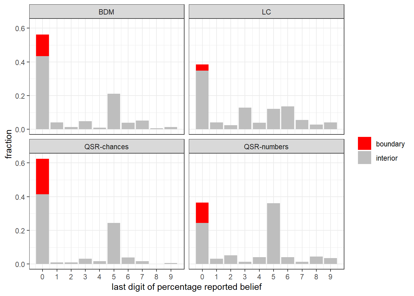
Figure 9.1: Last digit of reported belief in Holt and Smith (2016)
An important question when analyzing these data is how we should treat these data now that we know that there are lots of multiples of five and ten. One approach, which we (Yaroslav and I) have taken very seriously in James R. Bland and Rosokha (2025), is to treat the data as interval-valued. That is, if a participant (say) reported their answer as 60%, then we interpret it as having been rounded to 60%. As such, for this datum, we know that the participant’s actual answer (had they not rounded) was somewhere between 55% and 65%. We can motivate this as a “cost of decision-making” story: if the participant round to the nearest one (as they were forced to in Holt and Smith (2016)), then they have to choose between 101 different things. On the other hand, if they round to the nearest ten, then they are only choosing between eleven different things. Somewhere in the middle is rounding to five, where they chose between 21 different things. If we want to be really conservative (in James R. Bland and Rosokha (2025) we find that people are in fact more precise than this, particularly at the boundary) about what the data are telling us, we might adopt the following convention:
- If a participant’s decision is a multiple of ten, then it is assumed to be rounded to the nearest ten
- If a participant’s decision is a multiple of five (but not ten), then it is assumed to be rounded to the nearest five, and
- All other decisions are (forced by the experiment program) rounded to the nearest one.
And so a report of (say) \(x_{i,t}=60\) really only tells us that their real answer (if they didn’t round) was somewhere in the range \(x_{i,t}^*\in(55,65)\).
9.2.1 The Holt and Smith (2016) task
If you want to really understand this experiment, go and set yourself up on Veconlab and experiment on yourself with the “Bayes’ rule” experiment. For those of you who didn’t do this, here is a short explanation of the experiment:
A red cup conatins two red balls and one blue ball. A blue cup contains two blue balls and one red ball. Each cup is equally likely to be selected. We show you a number of draws with replacement from the selected cup, and you are incetivized to report your belief that the red cup is being used.
Holt and Smith (2016) investigate four different incentive schemes (between subjects) for eliciting beliefs. Each of them involves payoffs that depend on whether or not the red cup is being used.
- BDM “Becker-DeGroot-Marschak”: This mechanism binarizes the participant’s payoff. That is, they either earn $2 or $0 from their decision. Given the participant’s reported belief \(q\), the computer generates a random uniform number \(x\). If \(x\leq q\) then the participant is paid if the red cup is being used, otherwise the participant is paid if another random uniform number \(y<x\). This mechanism incentivizes truth-telling up to expected utility preferences (but does not incentivize truth-telling with (say) rank-dependent utility preferences).
- LC “Lottery choice”: Here, the participant is offered a series of binary choices between (i) a lottery that pays $2 with probability \(p\), and (ii) a lottery that pays $2 if the red cup was used. This mechanism elicits an indifference point (up to a coarsening of one percentage point) between options (i) and (ii).
- QSR-chances: This mechanism uses a quadratic scoring rule. The participant is paid a fixed amount, minus a quadratic loss function for placing probability on the incorrect event. That is, suppose the participant reports a belief of \(q\) that the red cup is being used. The loss term is proportional to \((1-q)^2\) if the red cup was actually used, and proportional to \(q^2\) if the blue cup was used. QSR incentivizes truth-telling if the participant has risk-neutral expected utility preferences. In the QSR-chances treatment, the decision problem was framed in terms of reporting probabilities.
- QSR-numbers: The same payoffs as the QSR-chances treatment, except the decision problem was not framed in terms of reporting probabilities.
9.2.2 A model for behavior in Holt and Smith (2016)
Here I will show you how to estimate a cut-down version of the Grether (1980) model.40 First, note that we can write the Bayesian belief in the red cup after observing signals (draws from the cup) \(s\) as:
\[ \begin{aligned} p(R\mid s)&=\frac{p(s\mid R)p(R)}{p(s)} \end{aligned} \]
Similarly, we can write the Bayesian belief in the blue cup after observing the same signals \(s\) as:
\[ \begin{aligned} p(B\mid s)&=\frac{p(s\mid B)p(B)}{p(s)} \end{aligned} \]
Taking the ratios of these, the pesky marginal likelihood \(p(s)\) cancels and we get:
\[ \begin{aligned} \frac{p(R\mid s)}{p(B\mid s)}&=\frac{p(s\mid R)p(R)}{p(s\mid B)p(B)} \end{aligned} \]
Now, in Holt and Smith (2016) \(p(R)=p(B)=0.5\), so we can write this as:
\[ \begin{aligned} \frac{p(R\mid s)}{p(B\mid s)}&=\frac{p(s\mid R)}{p(s\mid B)} \end{aligned} \]
And now we can put in a behavioral parameter \(\beta\) that measures how much the participant reacts to the the signal:
\[ \begin{aligned} \frac{p(R\mid s)}{p(B\mid s)}&=\left(\frac{p(s\mid R)}{p(s\mid B)}\right)^\beta \end{aligned} \]
Taking natural logs of both sides yields:
\[ \begin{aligned} \log p(R\mid s)-\log p(B\mid s)&=\beta\left[\log p(s\mid R)-\log p(s\mid B)\right] \end{aligned} \]
Finally, we add in an econometric error term:
\[ \begin{aligned} \overbrace{\log p(R\mid s)-\log p(B\mid s)}^{y_{i,t}}&=\beta\overbrace{\left[\log p(s\mid R)-\log p(s\mid B)\right]}^{\lambda_{i,t}} +\epsilon_{i,t} \end{aligned} \]
Therefore, \(\lambda_{i,t}\) is the (log) signal information associated with signal \(s_{i,t}\), and \(\beta\) measures departures from Bayesian updating, with \(\beta=1\) (and \(\epsilon_{i,t}=0\)) corresponding to the Bayesian benchmark. Here \(y_{i,t}\) is the “logit” of the participant’s belief. That is, \(\mathrm{logit}(x)=\log(x)-\log(1-x)\).
Note that this is a linear relationship, so in principle we could estimate this \(\beta\) using OLS (i.e. without a constant). However since our data are interval-valued, we would be violating an assumption needed for OLS to be valid. Instead, we will augment our data by the un-rounded latent beliefs.41
We will focus on estimating \(\beta\) for each participant in the experiment using a hierarchical model.
9.2.3 A note on replication
In this chapter, I am not trying to replicate Holt and Smith (2016). Neither am I trying to give you a “Bayesian version of Holt and Smith (2016)”. Rather, I am trying to use this dataset to show you how you can account for rounding and estimate the (cut-down version of the) Grether (1980) model using data augmentation. I have not run simulations (as we do in James R. Bland and Rosokha (2025)) to show (or not) that rounding is an important factor in this experiment, and my prior is that it won’t affect their conclusions substantially.42
9.2.4 Augmenting the data
We are going to augment our data in almost exactly the same way as we did with the probit model above. We will assume that participant \(i\)’s (logit) beliefs after seeing signal \(s_{i,t}\), but before any rounding, are represented by:
\[ \begin{aligned} y_{i,t}\mid s_{i,t}&\sim N(\beta_i \lambda_{i,t},\sigma_i^2) \end{aligned} \]
When we condition on the data, we truncate \(y_{i,t}\) to the bounds specified by the interval-valued data. For example, if our participant reported a belief of 60%, then we assume that this was rounded from the range of beliefs \([55%,65%]\), and since \(y_{i,t}\) is on the logit scale, we restrict it to \(y_{i,t}\in[\mathrm{logit}(0.55),\mathrm{logit}(0.65)]\approx[0.20,0.62]\). In Stan this is really easy: we just specify the lower and upper of y in the parameters block:
where y_lb and y_ub are these bounds (each are vector[N] data types), declared in the data block. From here, all we have to do is treat y as if it is data and give it a sampling statement in the model block, just as we would if we actually observed y:
Here is the hierarchical model I coded up in Stan to estimate this model:
data {

  int N; // number of observations in dataset
  int nParticipants;

  array[N] int participantID; // participant ID

  // lower and upper bounds of logit beliefs
  vector[N] y_lb;
  vector[N] y_ub;

  // log signal information
  vector[N] lambda;

  array[2] vector[2] prior_MU;
  vector[2] prior_TAU;
  real prior_Omega;

}


parameters {

  // population-level parameters -- one for each treatment
  vector[2] MU;
  vector<lower=0>[2] TAU;
  cholesky_factor_corr[2] L_Omega;

  // normalized participant-specific parameters
  matrix[2,nParticipants] z;

  vector<lower=y_lb,upper=y_ub>[N] y; // augmented data

}

transformed parameters {

  vector[nParticipants] beta;
  vector[nParticipants] sigma;

  {

    matrix[2,nParticipants] theta = rep_matrix(MU,nParticipants)
          + diag_pre_multiply(TAU,L_Omega)*z;

    beta = theta[1,]';
    sigma = exp(theta[2,]');

  }


}


model {

  //  hyper-prior --------------------------------------------------------------
  for (pp in 1:2) {
    MU[pp] ~ normal(prior_MU[pp][1],prior_MU[pp][2]);
    TAU[pp] ~ cauchy(0.0, prior_TAU[pp]);
  }
  L_Omega ~ lkj_corr_cholesky(prior_Omega);

  // hierarchical structure, non-centered parameterization ---------------------

  to_vector(z) ~ std_normal();

  // likelihood (augmented data) -----------------------------------------------

  y ~ normal(lambda.*beta[participantID],sigma[participantID]);

}

generated quantities {

  matrix[2,2] Omega = L_Omega*L_Omega';

  // convert the latent logit belief y variable into a probability
  vector[N] belief = inv_logit(y);


}
A word of caution might be worth making here. Note that this model has a lot of parameters. These are:
- 2 elements of
MU, the population mean vector - 2 elements of
TAU, the population standard deviation vector - 1 element of
L_Omega, the (Cholesky-factored) correlation matrix nParticipants\(\times 2\) participant-level parametersNelements of the augmented datay
It is the last one of these that we might want to worry about. N (the total number of decisions in the experiment) is typically large, so this means storing all of these latent quantities will take up a lot of RAM, and a lot of hard disk space if you save the results. I would argue, though, that we are not actually interested in these latent variables (what we really care about in are the estimates of \(\beta_i\)), and so we can just tell Stan to not store them using the par = "y", include = FALSE options when we call sampling in rstan. This also applies to the variable belief in the generated quantities block: there are N of these as well. However I want to save these so I can compare estimated un-rounded beliefs to reported beliefs in the experiment. My solution to avoid storing the entire posterior on my hard drive here is to just save Stan’s summary of the posterior distribution. In a lot of cases I have found that if you are forward-looking enough to get everything you want computed in the generated quantities block, this summary object is sufficient for most analysis.
9.2.5 Results
I estimate this model for each of the four treatments separately.
FitSum<-tibble()
D.beliefs<-tibble()

file.list<-list.files(path="Code/HS2016",pattern="fit_")

for (ff in file.list) {

  d<-paste0("Code/HS2016/",ff) |> read.csv()

  treat<-ff |> str_replace("fit_","") |> str_replace(".csv","")


  FitSum<-rbind(FitSum, d)

  d.beliefs<-d |>filter(grepl("belief",par)) |>
    mutate(
      reported.belief =  (D |> filter(treatment==treat))$Actual.Prediction/100,
      Actual.Prediction = (D |> filter(treatment==treat))$Actual.Prediction,
      Bayes..Prediction = (D |> filter(treatment==treat))$Bayes..Prediction,
      red.draws = (D |> filter(treatment==treat))$red.draws,
      blue.draws = (D |> filter(treatment==treat))$blue.draws,
      uid = (D |> filter(treatment==treat))$uid
    )

  D.beliefs<-rbind(D.beliefs,d.beliefs)


}
First, let’s compare the distribution of \(\beta_i\) between treatments. Here I will just plot the empirical cumulative density functions of the posterior means so that we can compare them in Figure 9.2:
dplt<-FitSum |>
  filter(grepl("beta",par))

(
  ggplot(dplt,aes(x=mean,color=treatment))
  +stat_ecdf(linewidth=1)
  +theme_bw()
  +geom_vline(xintercept=1, linetype="dashed")
  +xlab(expression(beta))
  +ylab("Empirical cumulative density of posterior means")
)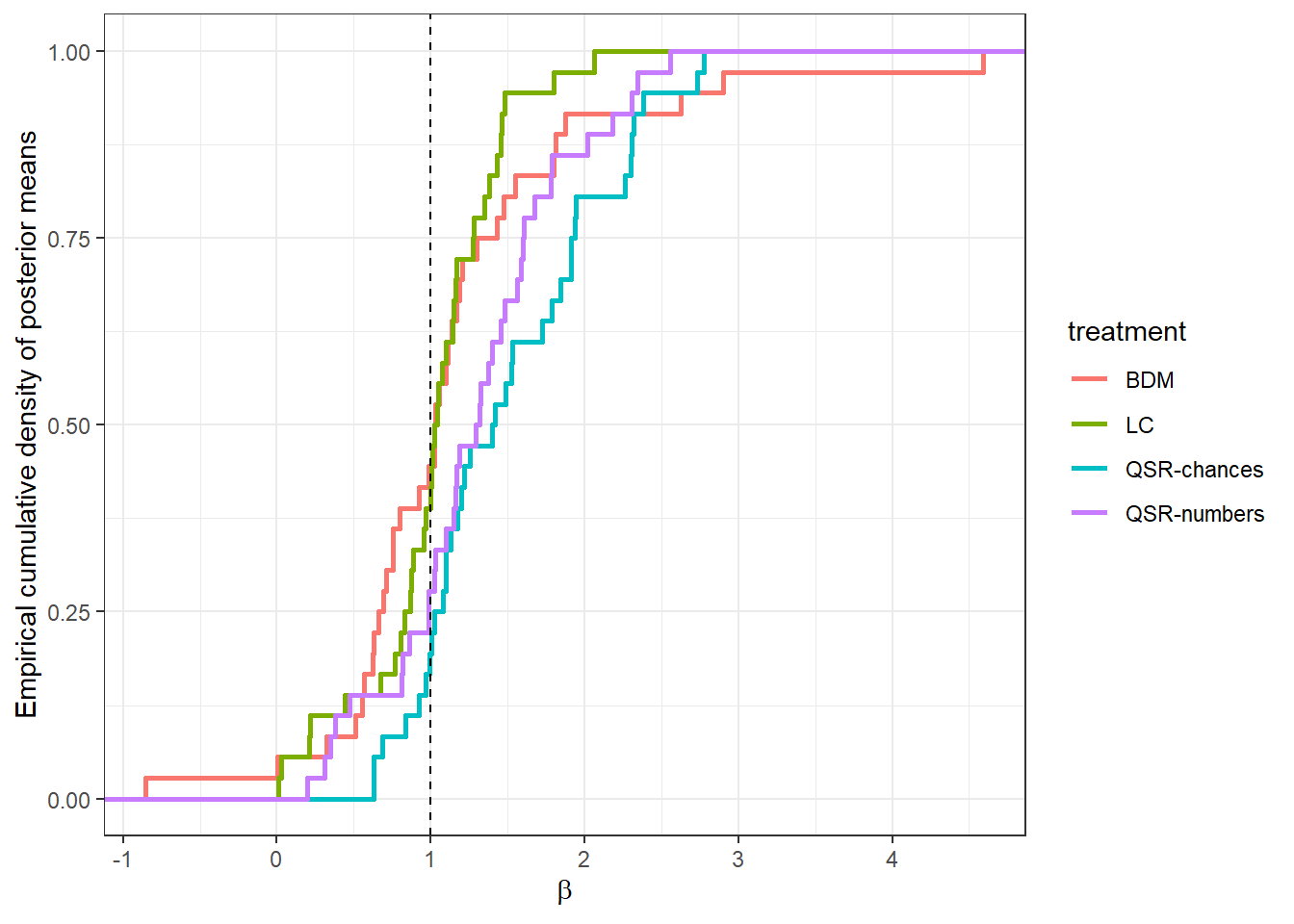
Figure 9.2: Empirical cumulative distribution functions of posterior means of \(\beta_i\) by treatment. The vertical dashed line is at \(\beta=1\), which is the Bayesian benchmark.
Overall, Figure 9.2 shows a wide range of updating behavior, including conservative (\(\beta<1\), under-reacting to the signal) and over-reaction \(\beta>1\), although the steepest part of the distributions (and hence their modes) seem to be at the Bayesian benchmark of \(\beta=1\). It looks like there is a longer tail at the “overreaction” end for the quadratic scoring rule (QSR, blue and purple) treatments.
param.names<-c("$\\beta$","$\\log\\sigma$")

fmt<-"%.3f"

TAB<-FitSum |>
  filter(
    grepl("MU",par) | grepl("TAU",par) | par=="Omega[2,1]"
  ) |>
  mutate(
    parameter = ifelse(grepl("MU",par),"mean ($\\mu$)",
                       ifelse(grepl("TAU",par),"sd ($\\tau$)","correlation ($\\Omega$)")
                       ),
    par.ind = par |> parse_number()
  ) |>
  pivot_longer(
    cols = c(mean,sd),
    names_to = "name",
    values_to = "value"
  ) |>
  mutate(
    value = ifelse(name=="mean",sprintf(fmt,value),paste0("(",sprintf(fmt,value),")"))
  ) |>
  arrange(treatment, par.ind,parameter,name) |>
  pivot_wider(
    id_cols = c(par.ind,name,parameter),
    names_from = treatment,
    values_from = value
  ) |>
  mutate(
    par.ind = param.names[par.ind]
  ) |>
  dplyr::select(-name) |>
  rename(
    `population quantity`=parameter,
    parameter = par.ind
  ) |>
  group_by(parameter,`population quantity`) |>
  mutate(
    `population quantity` = ifelse(row_number()==1,`population quantity`,"")
  ) |>
  group_by(parameter) |>
  mutate(
    parameter = ifelse(row_number()==1,parameter,"")
  )

TAB[is.na(TAB)]<-""

TAB |>
  kbl(caption = "Population-level estimates from the hierarchical models. Posterior means with posetrior standard deviations in parentheses.") |>
  kable_classic(full_width=FALSE) |>
add_header_above(c("","","treatment"=4))|
treatment
|
|||||
|---|---|---|---|---|---|
| parameter | population quantity | BDM | LC | QSR-chances | QSR-numbers |
| \(\beta\) | mean (\(\mu\)) | 1.135 | 1.018 | 1.508 | 1.293 |
| (0.172) | (0.092) | (0.129) | (0.127) | ||
| sd (\(\tau\)) | 0.972 | 0.493 | 0.673 | 0.671 | |
| (0.141) | (0.076) | (0.125) | (0.110) | ||
| \(\log\sigma\) | mean (\(\mu\)) | -0.717 | -1.012 | -0.465 | -0.412 |
| (0.183) | (0.185) | (0.153) | (0.173) | ||
| sd (\(\tau\)) | 1.070 | 1.085 | 0.877 | 1.013 | |
| (0.150) | (0.148) | (0.131) | (0.140) | ||
| correlation (\(\Omega\)) | 0.025 | 0.342 | 0.359 | 0.212 | |
| (0.181) | (0.156) | (0.152) | (0.169) | ||
Table 9.1 shows the posterior estimates of the population-level parameters for each treatment. Probably the ones of most interest are the ones that correspond to the distribution of \(\beta\), which are shown at the top of the table. Here we can see that the “LC” treatment has the closest mean to the Bayesian benchmark of \(\beta=1\), and it also the smallest standard deviation. The other treatments on average are in the overreaction direction (\(\beta>1\)), especially for the quadratic scoring rule treatments.
While the main goal of this example was to show you how we could estimate \(\beta_i\) and its population distribution using data augmentation, it is important to note that the augmented data itself may be useful in some circumstances, too. In our case, the inverse logit of the augmented ys are our models’ estimates of the participants’ un-rounded beliefs. One might wonder how much information these estimates are actually telling us. To see this, I plot the posterior interquartile ranges of the latent beliefs in Figure 9.3. This gives us an idea of how informative the model is for beliefs beyond the lower and upper bounds we passed to it for estimation. For example, for a decision that was rounded to ten percentage points, if the model was not particularly good at estimating these latent quantities, then the posterior for this latent belief might be uniformly distributed in the allowable range. In this case the interquartile range would be 0.05.43 The dashed vertical lines show the interquartile range we would see if the posterior distribution of latent beliefs are uniformly distributed in the allowable range. In fact, we see that almost all posteriors are at least as informative as this benchmark, showing that the model is somewhat able to pin down participants’ beliefs beyond just the range we provided Stan to begin with.
dplt<-D.beliefs |>
  mutate(
    rounding = ifelse((Actual.Prediction%%10)==0,"0.10",
                      ifelse((Actual.Prediction%%5)==0,"0.05","0.01")),
    IQR = X75.-X25.
  )

vlines<-tibble(
  rounding = c("0.10","0.05","0.01"),
  IQR = c(0.05, 0.025, 0.005)
)

(
  ggplot(dplt,aes(x=IQR,color=treatment))
  +stat_ecdf(linewidth=1)
  +geom_vline(data=vlines,aes(xintercept=IQR),linetype="dashed")
  +theme_bw()
  +facet_wrap(~rounding,scales="free")
  +xlab("posterior interquartile range of latent belief")
)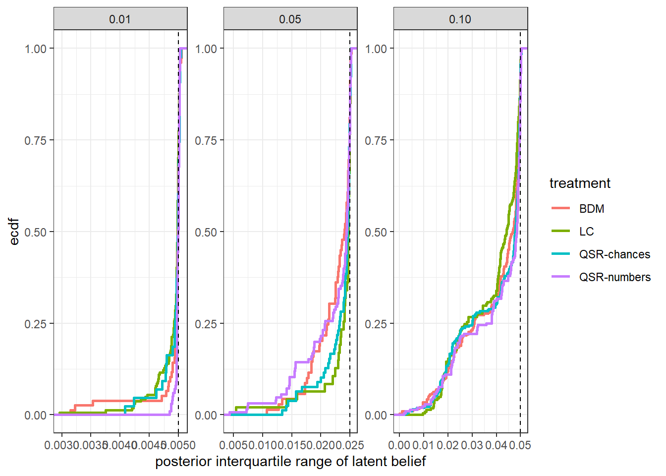
Figure 9.3: Posterior interquartile range of latent beliefs by rounding category. Vertical lines show the interquartile range if the posterior was uniformly distributed in the interval.
We can also look at the slice of the data corresponding to decisions where the participant made a particular rounded prediction of (say) 80%.44 For these decisions, we told our model that actual beliefs were somewhere between 75% and 85%. Figure 9.4 shows the distribution of these individual-level latent beliefs (the black line shows the empirical cumulative density of the posterior mean, and the red error bars show 50% Bayesian credible regions). While there is quite a range for these estimates, we can see that for some decisions participants’ latent beliefs were actually substantially different to 80% (based on their credible regions not overlapping with 80%).
dplt<-D.beliefs |>
  filter(Actual.Prediction==80) |>
  group_by(treatment) |>
  mutate(
    cumul = rank(mean)/n()-0.5/n()
  )

(
  ggplot(dplt)
  +stat_ecdf(aes(x=mean),linewidth=1)
  +geom_errorbar(aes(y=cumul,xmin=X25., xmax=X75.),color="red")
  +xlim(c(0.75,0.85))
  +facet_wrap(~treatment)
  +theme_bw()
  +xlab("Latent belief")
  +ylab("Empirical cumulative density of posterior mean")
)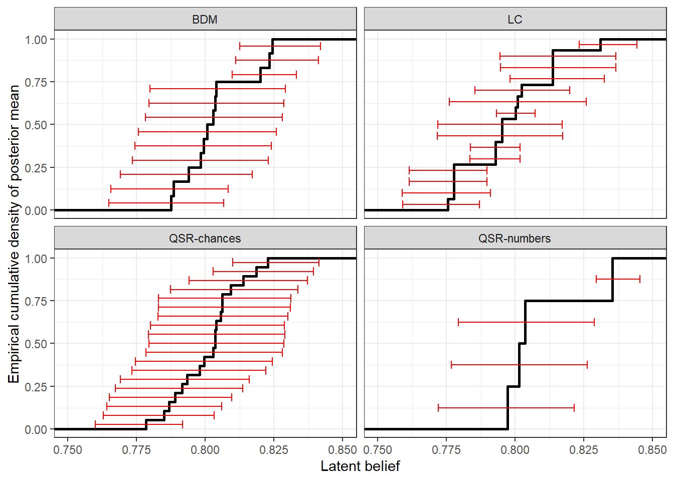
Figure 9.4: Posterior distribution of latent beliefs conditional on reporting a belief of 80%. Black line shows the empirical cumulative density of postterior means, and the red error bars show 50% Bayesian credible regions (25th-75th percentiles).
Finally, we can look at estimated beliefs after (say) observing one red ball and zero blue draws. In this case Bayes’ rule says that participants’ belief in the red cup being used should be \(\frac{2}{3}\). This is shows in Figure 9.5 as the black vertical dashed line. Here we can see that in all treatments there is some spread around this true value, although there is less spread in the BDM and LC treatments, with a substantial mass choosing very close to the correct number.
dplt<-D.beliefs |>
  filter(
    red.draws==1 & blue.draws==0
  ) |>
  group_by(treatment) |>
  mutate(
    cumul = rank(mean)/n()-0.5/n()
  )

(
  ggplot(dplt)
  +stat_ecdf(aes(x=mean))
  +facet_wrap(~treatment)
  +geom_point(aes(x=reported.belief,y=cumul),size=1,color="blue")
  +geom_errorbar(aes(y=cumul,xmin = X25., xmax=X75.),color="red")
  +geom_vline(xintercept=2/3,color="black",linetype="dashed")
  +theme_bw()
  +xlab("Belief in red cup")
  +ylab("Empirical cumulative density of posterior mean")
)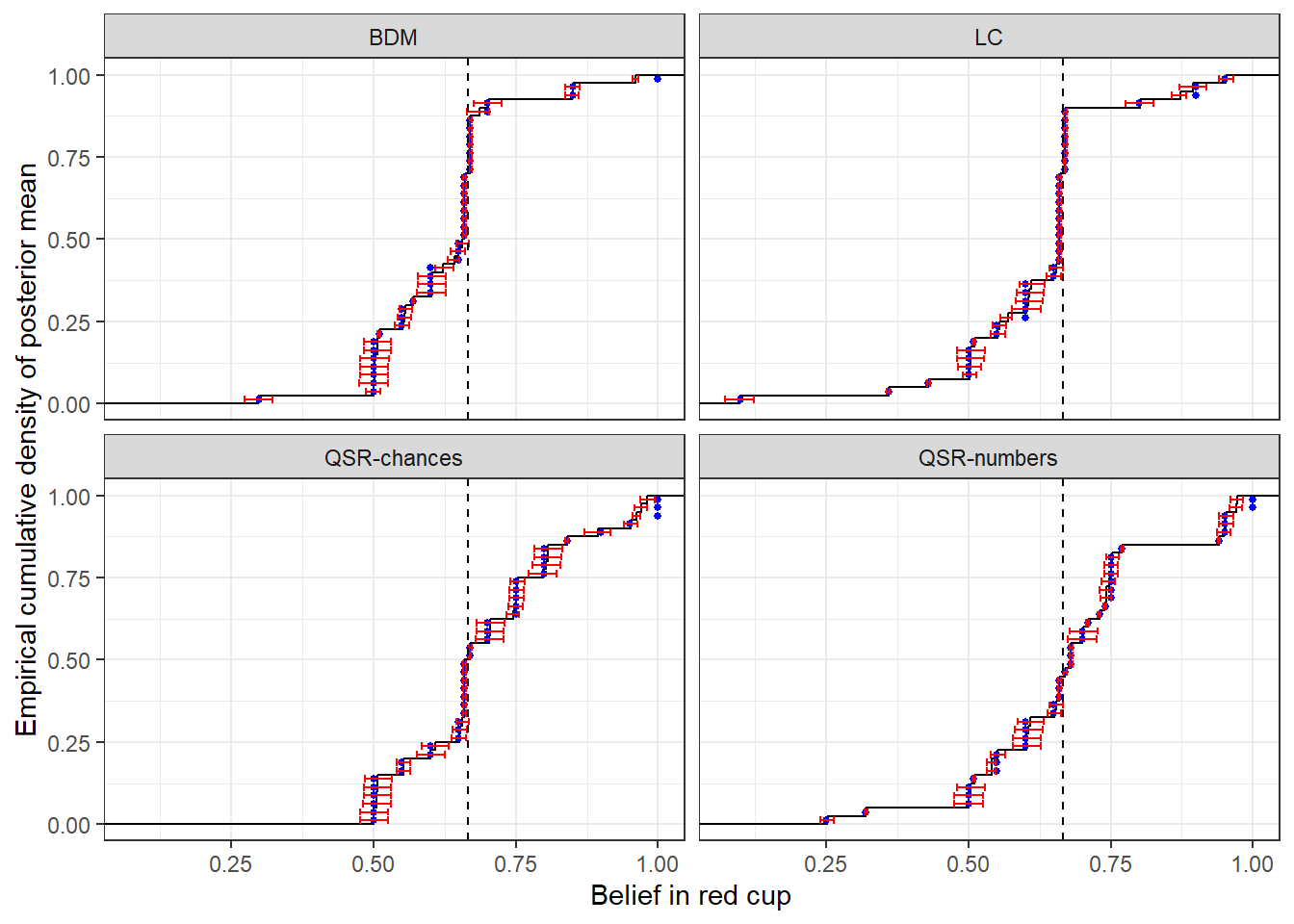
Figure 9.5: Distribution of latent beliefs after observing one red ball. Black line shows the empirical cumulative density function of posterior means. Red error bars show 25% Bayesian credible regions (25th-75th percentiles). Blue dots show reported belief.
9.3 R code used for this chapter
9.3.1 Loading the data
library(tidyverse)
library(readxl)

D<-tibble()

for (tt in c("LC","BDM","QSR-chances","QSR-numbers")) {
  D<-D |> rbind(
      "Data/HS2016/RawData_AEJMicro-2013-0274.R2.xls" |>
        read_excel(sheet=tt) |>
        mutate(treatment = tt) |>
        select(treatment,Session,Round,ID,`1st Draw`,`2nd Draw`, `3rd Draw`,`4th Draw`,`Bayes' Prediction`,`Actual Prediction`)
  )
}

D<-D |>
  mutate(
    red.draws =(`1st Draw`=="r")+(`2nd Draw`=="r")+(`3rd Draw`=="r")+(`4th Draw`=="r"),
    blue.draws = (`1st Draw`=="b")+(`2nd Draw`=="b")+(`3rd Draw`=="b")+(`4th Draw`=="b")
  )

dplt<- D|>
  group_by(treatment,`Bayes' Prediction`,`Actual Prediction`) |>
  summarize(count=n())

(
  ggplot(dplt,aes(x=`Bayes' Prediction`,y=`Actual Prediction`))
  +geom_point(aes(size=count))
  +facet_wrap(~treatment)
  +theme_bw()
  +geom_abline(slope=1,intercept=0,color="red")
  +geom_smooth(data=D)
)

D |>
  write.csv("Code/HS2016/cleaneddata.csv")
9.3.2 Estimating the models
library(tidyverse)
library(rstan)
options(mc.cores = parallel::detectCores())
rstan_options(auto_write = TRUE)

D<-"Code/HS2016/cleaneddata.csv" |>
  read.csv() |>
  mutate(
      net.red.draws = red.draws-blue.draws,
      lambda = log((2/3)/(1/3))*net.red.draws,

      belief = Actual.Prediction/100,

      belief.lb = ifelse((Actual.Prediction %% 10)==0, belief-0.05,
                         ifelse((Actual.Prediction) %% 5 ==0, belief-0.025,
                                belief-0.005
                         )
      ),
      belief.ub = ifelse((Actual.Prediction %% 10)==0, belief+0.05,
                         ifelse((Actual.Prediction) %% 5 ==0, belief+0.025,
                                belief+0.005
                         )
      ),

      y.lb = log(belief.lb)-log(1-belief.lb),
      y.ub = log(belief.ub)-log(1-belief.ub),

      y.lb = ifelse(belief.lb<=0,-Inf,y.lb),
      y.ub = ifelse(belief.ub>=1,Inf,y.ub),

      uid = paste(Session,ID,treatment) |> as.factor() |> as.numeric()
    ) |>
  group_by(treatment) |>
  mutate(
    uid.treatment = paste(Session,ID,treatment) |> as.factor() |> as.numeric()
  )

id.lookup<-D |>
  group_by(Session, ID, treatment) |>
  summarize(
    uid = mean(uid),
    uid.treatment = mean(uid.treatment)
  ) |>
  arrange(uid)

id.lookup |>
  write.csv("Code/HS2016/idlookup.csv")

model <-"Code/HS2016/hierarchical_single_treatment.stan" |>
  stan_model()


for (tt in unique(D$treatment)) {

  print(tt)

  file<-paste0("Code/HS2016/fit_",tt,".csv")

  if (!file.exists(file)) {
    d<-D |>
      filter(treatment==tt)

    dStan<-list(
      N = dim(d)[1],
      nParticipants = d$uid.treatment |> unique() |> length(),

      participantID = d$uid.treatment,

      y_lb = d$y.lb,
      y_ub = d$y.ub,
      lambda = d$lambda,

      prior_MU = list(
        c(1,1),
        c(0,1)
      ),
      prior_TAU = c(1,1),
      prior_Omega = 4
    )

    Fit<-model |>
      sampling(
        data=dStan,
        seed=42,
        # I was getting some ESS warnings with the default settings
        iter = 20000, chains = 16,
        # I was getting some divergent transitions warnings with the default settings
        control = list(adapt_delta=0.999),
        #iter = 100, chains = 1, # debug settings
        include = FALSE, par = c("y","z","L_Omega"),
        init_r = 0.1
      )

    Fit |> check_hmc_diagnostics()

    summary(Fit)$summary |>
      data.frame() |>
      rownames_to_column(var="par") |>
      mutate(treatment=tt) |>
      write.csv(file)

    tibble(
      MU.beta = extract(Fit)$MU[,1],
      TAU.beta = extract(Fit)$TAU[,1],
      treatment = tt
    ) |>
      write.csv(paste0("Code/HS2016/beta_hyperposterior_",tt,".csv"))


  }


}
References
By this, I mean the art of deriving conjugate priors for everything and coding up one’s own Gibbs sampler.↩︎
Go and read James R. Bland and Rosokha (2025) for how to do the full thing, complete with how to implement it in Stan. ↩︎
We could, however, estimate this with interval regression. ↩︎
This is because in James R. Bland and Rosokha (2025) we find that rounding at the boundary is really important. There just aren’t that many boundary decisions in Holt and Smith (2016), and so I don’t think our treatment of rounding is going to change their conclusions. ↩︎
For example, if a participant reports beliefs of 70%, then we pass bounds for their latent beliefs to Stan as (the logit of) \([0.65,0.75]\). If the posterior latent belief is uniformly distributed in this range, then the posterior interquartile range will be 0.05.↩︎
I chose this because these reports were fairly common in the data. The most common report was 50%, but I wanted to focus on data that were not associated with just eliciting the prior probability of the red cup. ↩︎