22 Application: Estimating game payoffs using Quantal Response Equilibrium

While we usually know our (monetary) payoffs for sure in economic experiments because we choose them ourselves, it is common in another field that uses a lot of structural estimation to estimate them. Here, I am referring to structural industrial organization (IO), where the payoffs, or payoff parameters, to be estimated are often (say) payoffs in entry games, cost functions, and so on. While the IO people will most likely never be able to validate their estimates against their true values (because firms usually want to hide these things), as experimentalists, we can!. In particular, becuase we have set the payoffs in our game, we can work out whether or not a particular econometric technique recovers the parameters well or not.

In this chapter I will show you some logit quantal response equilibrium models where we leave some of the payoff parameters as unknown quantities to be estimated. Once we have a QRE model that works with all of the payoffs are known, this is really easy: just move the the unknown parameters from the data block to the parameters block and assign appropriate priors! Whether the model actually recovers the parameters well is, of course, a function of the data-generating process as well, and we can investigate this with simulation.

22.1 Example dataset and model

Holt and Palfrey (2024) study the attacker-defender game shown in Table 22.1. In a within-subjects design, participants played 20 rounds of this game with fixed matchings, then played another 20 rounds matched with the same participant, but with different payoffs.

U<-rbind(c("-a, a", "-c, c"),c("-b, b", "-d, d"))
rownames(U)<-c("Top", "Bottom")
colnames(U)<-c("Left", "Right")

U |>
  kbl(caption = "Payoff matrix of attacker-defender game studied by @HP2024. $b>a>0$, $c>d>0$, $c>a$, $b>d$") |>
  kable_classic(full_width=FALSE)

Table 22.1: Payoff matrix of attacker-defender game studied by Holt and Palfrey (2024). \(b>a>0\), \(c>d>0\), \(c>a\), \(b>d\)

	Left	Right
Top	-a, a	-c, c
Bottom	-b, b	-d, d

Like Holt and Palfrey (2024), we will be analyzing these data through the lens of Nash equilibrium and Quantal Response equilibrium. The Nash equilibrium is unique and in mixed strategies, which is: \[ \begin{aligned} p^\mathrm{Top}&=\frac{b-d}{b-d+c-a}\\ p^\mathrm{Left}&=\frac{c-d}{c-d+b-a} \end{aligned} \]

For Quantal Response Equilibrium, we can write the equilibrium condition as:

\[ \begin{aligned} 0&=\log (p^\mathrm{Top})-\log(1-p^\mathrm{Top})-\lambda \begin{pmatrix} 1 & -1\end{pmatrix}U\begin{pmatrix} p^\mathrm{Left} \\ 1- p^\mathrm{Left}\end{pmatrix}\\ 0&=\log (p^\mathrm{Left})+\log(1-p^\mathrm{Left})+\lambda \begin{pmatrix} 1 & -1\end{pmatrix}U^\top\begin{pmatrix} p^\mathrm{Top} \\ 1- p^\mathrm{Top}\end{pmatrix}\\ \text{where: }U&=\begin{bmatrix} -a & -c \\ -b & -d \end{bmatrix} \end{aligned} \]

However, as mentioned in the previous QRE chapters, it is best to not solve for QRE in mixed strategy levels. For this application I found that solving for QRE on the logit scale worked very well, and only required constant-\(\lambda\) Newton steps. So we re-write the above system as:

\[ \begin{aligned} 0&=\ell^\mathrm{Top}-\lambda \begin{pmatrix} 1 & -1\end{pmatrix}U\begin{pmatrix} p^\mathrm{Left} \\ 1- p^\mathrm{Left}\end{pmatrix}\\ 0&=\ell^\mathrm{Left}+\lambda \begin{pmatrix} 1 & -1\end{pmatrix}U^\top\begin{pmatrix} p^\mathrm{Top} \\ 1- p^\mathrm{Top}\end{pmatrix} \end{aligned} \]

where \(p^X=\Lambda(\ell^X)\) and \(\Lambda(y)=(1+\exp(-y))\) is the inverse logit function. So we can stack these into one function as: \[ \begin{aligned} H(\ell;\lambda)&=\begin{pmatrix} \ell^\mathrm{Top}-\lambda \begin{pmatrix} 1 & -1\end{pmatrix}U\begin{pmatrix} p^\mathrm{Left} \\ 1- p^\mathrm{Left}\end{pmatrix} \\ \ell^\mathrm{Left}+\lambda \begin{pmatrix} 1 & -1\end{pmatrix}U^\top\begin{pmatrix} p^\mathrm{Top} \\ 1- p^\mathrm{Top}\end{pmatrix} \end{pmatrix} \end{aligned} \]

Noting that \(\Lambda'(y)=\Lambda(y)(1-\Lambda(y))\), we can write the Jacobian of the system as:

\[ J(\ell;\lambda)=\begin{bmatrix} 1 & -\lambda \begin{pmatrix} 1 & -1\end{pmatrix}U\begin{pmatrix} 1 \\ -1\end{pmatrix}p^\mathrm{Left}(1-p^\mathrm{Left})\\ \lambda \begin{pmatrix} 1 & -1\end{pmatrix}U^\top\begin{pmatrix} 1 \\ -1\end{pmatrix}p^\mathrm{Top}(1-p^\mathrm{Top})&1 \end{bmatrix} \]

So the Newton steps to solve for QRE at a given choice precision \(\lambda\) are just:

\[ \ell_{t+1}=\ell_t-J(\ell_t;\lambda)^{-1}H(\ell_t;\lambda) \]

Since we will be solving this a lot below, in a lot of different Stan files, I wrote a user-defined function to include in all of the programs I wrote:

  vector lpQRE(
    real lambda,
    real a, real b, real c, real d,
    data int maxiter, data real tol
  ) {
    
    /* This function solves QRE in the logit space
    */
    
    matrix[2,2] Urow = [[-a, -c],[-b,-d]];
    matrix[2,2] Ucol = -Urow';
    
    // initialization
    vector[2] logitp = [0.0,0.0]';
    
    for (ii in 1:maxiter) {
      
      vector[2] p = inv_logit(logitp);
      vector[2] p1mp = p.*(1.0-p);
      
      // zero function
      vector[2] H;
      H[1] = logitp[1]-lambda*[1.0, -1.0]*Urow*[p[2],1.0-p[2]]';
      H[2] = logitp[2]-lambda*[1.0, -1.0]*Ucol*[p[1],1.0-p[1]]';
      
      // Jacobian
      matrix[2,2] J = diag_matrix([1.0,1.0]');
      J[1, 2] += -lambda*[1.0, -1.0]*Urow*[p1mp[2],-p1mp[2]]';
      J[2, 1] += -lambda*[1.0, -1.0]*Ucol*[p1mp[1],-p1mp[1]]';
      
      vector[2] dlogitp = -J\H;
      logitp += dlogitp;
      
      if (max(abs(dlogitp))<tol) {
        break;
      }
      
      if (ii == maxiter) {
        reject("maxiter reached, lambda =",lambda);
      }
      
    }
    
    return(logitp);
    
  }

I add this to the `functions’ block for all of my Stan programs. For example, here is the program for estimating the basic logit QRE model with known payoff parameters:

functions {
  
  
  #include input_QREsolver.stan
  
}

data {
  
  int nTreat; // number of treatments
  
  vector[nTreat] A, B, C, D;
  
  array[nTreat] int count, top, left;
  
  int<lower=0, upper=1> UseData;
  
  vector[2] prior_lambda;
  
  int<lower=1> maxiter;
  real<lower=0> tol;
  
}


parameters {
  
  real<lower=0> lambda;
  
}

transformed parameters {
  
  array[nTreat] vector[2] logitp;
  
  vector[nTreat] pTop, pLeft;
  
  for (tt in 1:nTreat) {
    logitp[tt] = lpQRE(
    lambda,
    A[tt],B[tt],C[tt],D[tt],
    maxiter, tol
    );
    
    pTop[tt] = inv_logit(logitp[tt][1]);
    pLeft[tt] = inv_logit(logitp[tt][2]);
  }
  
}


model {
  
  lambda ~ lognormal(prior_lambda[1], prior_lambda[2]);
  
  if (UseData==1) {
    for (tt in 1:nTreat) {
    
      
      top[tt] ~ binomial_logit(count[tt], logitp[tt][1]);
      left[tt] ~ binomial_logit(count[tt], logitp[tt][2]);
    }
  }
  
  
  
}

Importantly here, I have the data element `UseData’, which lets me turn on or off the likelihood contribution. This is particularly useful for doing a prior calibration, because we can use the same Stan program to get both prior and posterior simulations. Additionally, note that the data passed to Stan is in count form, collapsed by treatment. This means the sampler only has to compute QRE four times (once per treatment), rather than (say) once per played game.

22.2 Prior check

Before estimating anything, it is always worthwhile spending some time thinking about the prior. To begin with, I computed the logit QRE correspondence for a wide range of \(\lambda\), which can be seen in Figure 22.1. This is helpful because it gives you a sense of the sale of \(\lambda\): for example, we can determine what values of \(\lambda\) make similar-enough predictions to \(\lambda=0\), or Nash equilibrium (\(\lambda\to\infty\)). Here I decided that I wanted \(\lambda\approx 0.3\) to be about in the middle of the prior, so for a log-normal prior this sets the location parameter of the prior to \(\log0.3\).

priorcheck<-"Code/HP2024/lambda_prior_check.csv" |>
  read.csv() |>
  dplyr::select(
    lambda.sd, lambda, contains("Top"), contains("Left"), simstep
  ) |>
  pivot_longer(
    cols = pTop.1.:pLeft.3.,
    names_to = "name",
    values_to = "prob"
  ) |>
  mutate(
    action = ifelse(grepl("Top",name), "Top","Left"),
    treatment.id = 10*(name |>  parse_number())
  ) |>
  full_join("Code/HP2024/collapsed_data.csv" |>
              read.csv(),
            by = "treatment.id"
            ) |>
  mutate(
    treatment.txt = paste0("a = ",a,", b = ",b),
    lambda.sd.txt = paste0("sd(\u03bb) = ", lambda.sd),
    lambda.sd.txt.factor = forcats::fct_reorder(lambda.sd.txt, parse_number(lambda.sd.txt))
  )

(
  ggplot(priorcheck, aes(x=lambda, y=prob, color=treatment.txt))
  +geom_line(linewidth=1)
  +facet_grid(action~.)
  +scale_x_continuous(trans="log10")
  +theme_bw()
  +xlab(expression(lambda))
  +ylab("QRE mixed strategy")
  +coord_cartesian(xlim = c(1e-2,1e2))
  +scale_color_manual(name = "treatment",values = c("black", "red", "blue"))
)

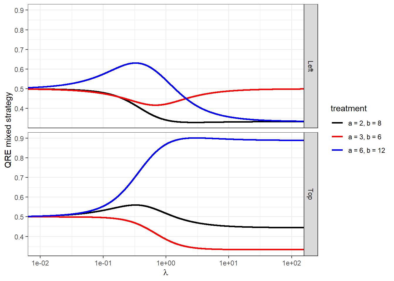
Figure 22.1: Quantal response equilibrium corresponsence as a function of \(\lambda\).

But what about the scale parameter? Since the model is highly non-linear, it is not clear at first glance that setting this scale parameter to a large number is a good idea. In particular, if we pick a really large scale parameter for this prior, then almost 50% of the prior mass will be close enough to \(\lambda = 0\) (say, \(\lambda<10^{-2}\)) that participants will just be flipping fair coins, and 50% of the prior mass will be “near enough” to infinity (say, \(\lambda>1,000\)) that participants will be effectively be playing Nash equilibrium. Figure 22.2 plots posterior simulations of the logit QRE locus for the three distinct treatment for four different values of the scale parameter. The locus is the set of mixed strategies that constitute a QRE for any choice precision. Here you can see that \(\mathrm{sd}(\lambda)=1\) is probably too small, so there is not good coverage of the endpoints of the locus (both at 50-50 randomization and Nash), while \(\mathrm{sd}(\lambda)=27\) only really covers parts of the locus that are close to these endpoints. In the end, I chose \(\mathrm{sd}(\lambda)=3\) as my prior, which has reasonably good coverage of the entire logit QRE locus.

d<-"Code/HP2024/collapsed_data.csv" |>
              read.csv() |>
  mutate(
    pTop = top/count,
    pLeft = left/count,
    treatment.txt = paste0("a = ",a,", b = ",b)
  )

dplt<-priorcheck |>
  pivot_wider(
    id_cols = c(simstep,lambda, lambda.sd, lambda.sd.txt.factor, treatment.txt, treatment.id), 
    names_from = action, 
    values_from = prob
  )

(
  ggplot(dplt, aes(x=Top, y=Left, color = treatment.txt))
  +geom_jitter(size=0.1, width=0.005, height=0.0005, alpha=0.1)
  +geom_text(data=d, aes(x=pTop, y=pLeft,label="X"))
  +facet_wrap(~lambda.sd.txt.factor)
  +theme_bw()
  +guides(color = guide_legend(override.aes = list(size = 3, alpha = 1)))
  +scale_color_manual(name = "treatment",values = c("black", "red", "blue"))
)

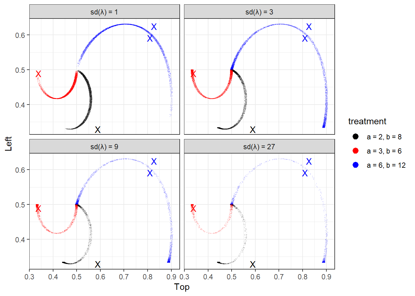
Figure 22.2: QRE locus coverage for different choices of the prior standard deviation for \(\lambda\). Each dot is a draw from the prior simulation, with the coordinates jittered slightly for clarity. Points marked ‘X’ show treatment means choice frequencies.

22.3 Estimation with known payoffs

First, I start with estimating the logit QRE model with known payoffs. That is, \(\lambda\) is the only free parameter. Before looking at the posterior distribution of \(\lambda\) itself, I find it more useful to look at the posterior distribution of estimated mixed strategies along the locus.¹⁰² This is shown in Figure 22.3.

Fit<-"Code/HP2024/Fit_QRE_known_parameters.rds" |>
  readRDS() |>
  as.data.frame() |>
  dplyr::select(lambda, contains("Top"), contains("Left")) |>
  mutate(
    simstep = 1:n()
  ) |>
  pivot_longer(
    cols = `pTop[1]`:`pLeft[4]`,
    names_to = "name",
    values_to = "prob"
  ) |>
  mutate(
    action = ifelse(grepl("Top",name), "Top","Left"),
    treatment.id = name |>  parse_number()
  ) |>
  full_join("Code/HP2024/collapsed_data.csv" |>
              read.csv(),
            by = "treatment.id"
            ) |>
  mutate(
    treatment.txt = paste0("a = ",a,", b = ",b)
  ) |>
  pivot_wider(
    id_cols = c(simstep,lambda, treatment.txt, treatment.id), 
    names_from = action, 
    values_from = prob
  )

pc <- priorcheck |>
  pivot_wider(
    id_cols = c(simstep, treatment.id, treatment.txt, lambda),
    names_from = action, 
    values_from =prob
  ) |>
  arrange(lambda) |>
  filter(!is.na(Left))
  

(
  ggplot(Fit, aes(x=Top, y=Left, color = treatment.txt))
  +geom_jitter(size=0.1, width=0.005, height=0.0005, alpha=0.1)
  +geom_path(data=pc)
  +geom_text(data=d, aes(x=pTop, y=pLeft,label="X"))
  +theme_bw()
  +guides(color = guide_legend(override.aes = list(size = 3, alpha = 1)))
  +scale_color_manual(name = "treatment",values = c("black", "red", "blue"))
)

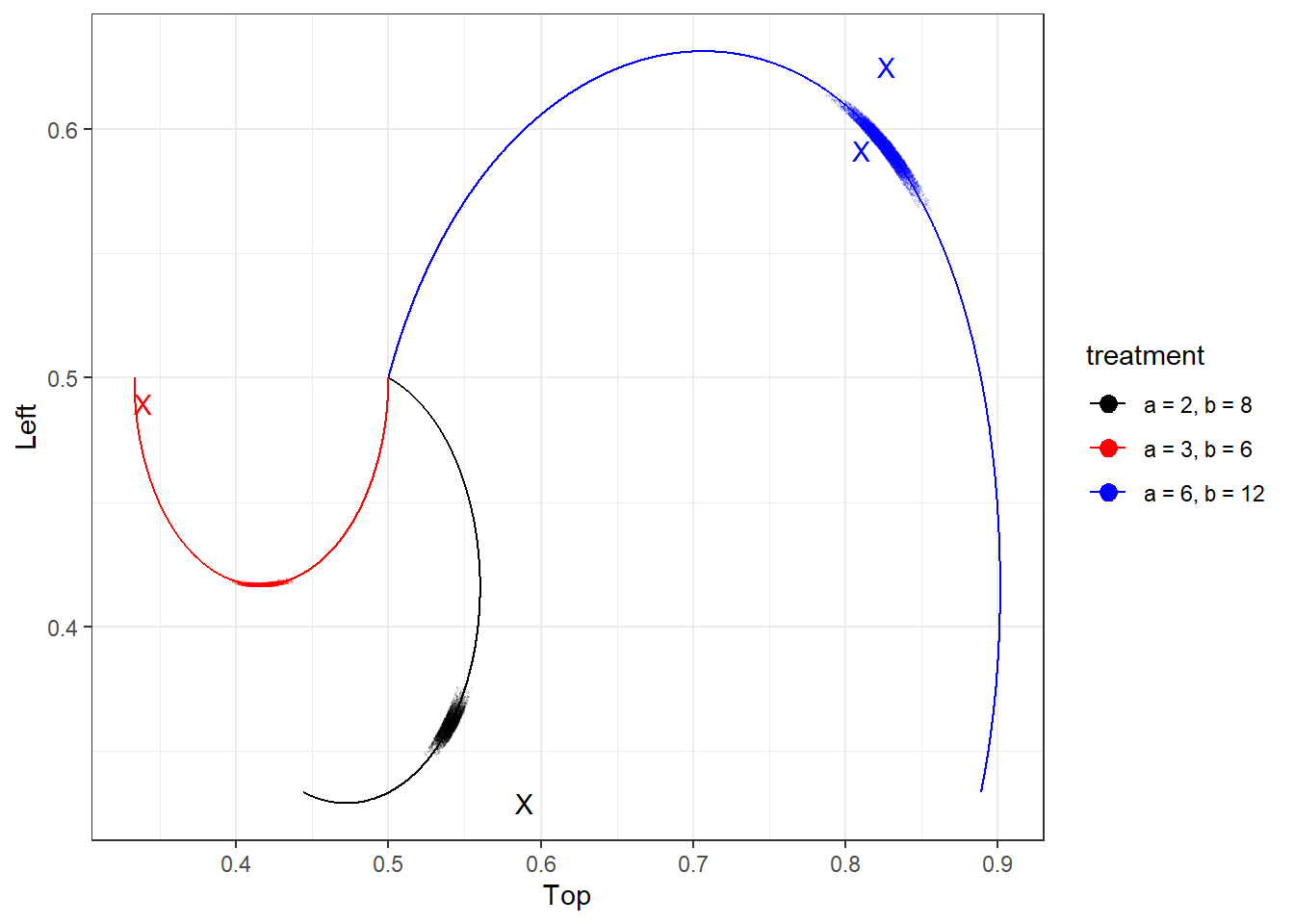
Figure 22.3: Posterior locus coverage of the homogeneous logit QRE with known payoffs

Figure 22.4 shows the posterior distribution of \(\lambda\) from this model. Holt and Palfrey (2024) estimate \(\lambda=0.7\) using MLE. Since my prior median is slightly below this (at 0.3), it is unsurprising that my estimate comes in a little bit lower.

(
  ggplot()
  +geom_density(data=Fit |> filter(treatment.id==1), aes(x=lambda),linewidth=1)
  +theme_bw()
  #+scale_x_continuous(trans="log10")
  +xlab(expression(lambda))
)

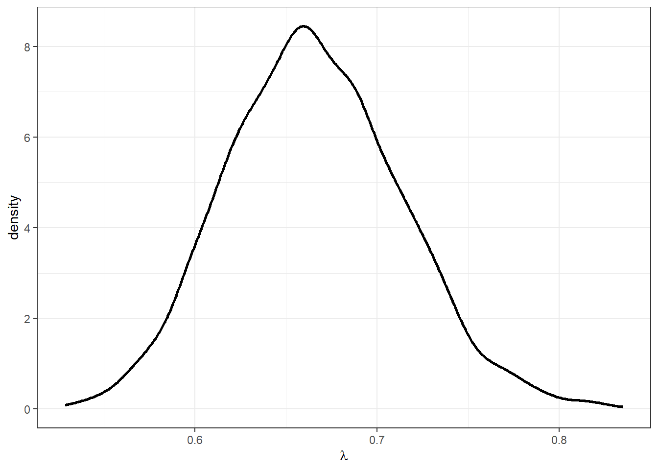
Figure 22.4: Posterior distribution of logit choice precision \(\lambda\)

22.4 Estimation with unknown payoffs

Now we can move to the industrial organization-y task of trying to estimate the payoffs in the game. But since these payoffs were known, we can use this as a model-validation exercise to see how well our models recover the parameters. Holt and Palfrey (2024) focus on how well the model recovers the parameters \(c\) and \(d\) while knowing the values of \(a\) and \(b\). Since \(c=7\) and \(d=4\) were common to all treatments, this means estimating two additional parameters. I will do this estimation task, as well as a separate task of estimating \(a\) and \(b\), which are treatment-specific, when \(c\) and \(d\) are known. This is a harder task because there are four values of each of these parameters. Furthermore, Holt and Palfrey (2024) for this estimation assume that \(\lambda\) is fixed at \(0.70\) (their maximum likelihood estimate), whereas I will treat \(\lambda\) as a free parameter. We will have to be careful here, though, becuase we have an identification problem. For example, the model makes the same predictions if (say) we double \(\lambda\) and halve all of the payoff parameters. Therefore, it is important to keep at least one of the four payoff parameters known.

22.4.1 Unknown \(c\) and \(d\)

To begin with I follow Holt and Palfrey (2024) and estimate \(c\) and \(d\) assuming Nash equilibrium and logit QRE, however for logit QRE I allow \(\lambda\) to also be a free parameter. This basically comes down to moving a and b from the data block to the parameters block. I adopt a uniform prior over these parameters, with an upper bound of 20. Here is the Stan program I wrote to estimate this model:

functions {
  
  
#include input_QREsolver.stan
  
}

data {
  
  int nTreat; // number of treatments
  
  vector[nTreat] A, B;
  
  array[nTreat] int count, top, left;
  
  int<lower=0, upper=1> UseData;
  
  vector[2] prior_lambda;
  
  int<lower=1> maxiter;
  real<lower=0> tol;
  
  real<lower=0> payoffUB;
  
}


parameters {
  
  real<lower=0, upper=payoffUB> c, d;
  
  real<lower=0> lambda;
  
}

transformed parameters {
  
  array[nTreat] vector[2] logitp;
  
  vector[nTreat] pTop, pLeft;
  
  for (tt in 1:nTreat) {
    logitp[tt] = lpQRE(
    lambda,
    A[tt],B[tt],c,d,
    maxiter, tol
    );
    
    pTop[tt] = inv_logit(logitp[tt][1]);
    pLeft[tt] = inv_logit(logitp[tt][2]);
  }
  
}


model {
  
  lambda ~ lognormal(prior_lambda[1], prior_lambda[2]);
  
  if (UseData==1) {
    for (tt in 1:nTreat) {
    
      
      top[tt] ~ binomial_logit(count[tt], logitp[tt][1]);
      left[tt] ~ binomial_logit(count[tt], logitp[tt][2]);
    }
  }
  
  
  
}

And for Nash equilibrium, I just moved \(\lambda\) to the data block and set it equal to a very large number (1,000 seemed like enough):

functions {
  
  
#include input_QREsolver.stan
  
}

data {
  
  int nTreat; // number of treatments
  
  vector[nTreat] A, B;
  
  array[nTreat] int count, top, left;
  
  int<lower=0, upper=1> UseData;
  
  vector[2] prior_lambda;
  
  int<lower=1> maxiter;
  real<lower=0> tol;
  
  real<lower=0> payoffUB;
  
  real<lower=0> lambda;
}


parameters {
  
  real<lower=0, upper=payoffUB> c, d;
  
  
  
}

transformed parameters {
  
  array[nTreat] vector[2] logitp;
  
  vector[nTreat] pTop, pLeft;
  
  for (tt in 1:nTreat) {
    logitp[tt] = lpQRE(
    lambda,
    A[tt],B[tt],c,d,
    maxiter, tol
    );
    
    pTop[tt] = inv_logit(logitp[tt][1]);
    pLeft[tt] = inv_logit(logitp[tt][2]);
  }
  
}


model {
  
  if (UseData==1) {
    for (tt in 1:nTreat) {
    
      
      top[tt] ~ binomial_logit(count[tt], logitp[tt][1]);
      left[tt] ~ binomial_logit(count[tt], logitp[tt][2]);
    }
  }
  
  
  
}

22.4.1.1 Parameter recovery check

Before diving into the estimation, it is important to have an idea about how accurate our estimator will be. That is, we can simulate data with a known data-generating process, and see if we have any chance at all of recovering the parameters. For this, I use draws from the prior to simulate data, so this will give us a good variation in \(\lambda\) over the relevant range. Figure 22.5 shows how well the two payoff parameters are recovered. This mostly looks good, except for being imprecisely estimated and poorly calibrated for a substantial minority of simulated samples.

dplt<-"Code/HP2024/param_recovery.csv" |>
  read.csv()|>
  filter(parameter=="c" | parameter =="d") |>
  group_by(
    parameter
  ) |>
  mutate(
    rank = rank(mean)/(n())
  )

(
  ggplot(dplt,aes(x=rank, y=mean))
  +geom_point()
  +geom_errorbar(aes(ymin = X25., ymax = X75.))
  +facet_grid(parameter~., scales="free")
  +geom_hline(aes(yintercept=truth), color="red", linetype="dashed")
  +theme_bw(
  )
  +theme(
    axis.title.x = element_blank(),
    axis.text.x  = element_blank(),
    axis.ticks.x = element_blank()
  )
  +ylab("estimate")
  
)

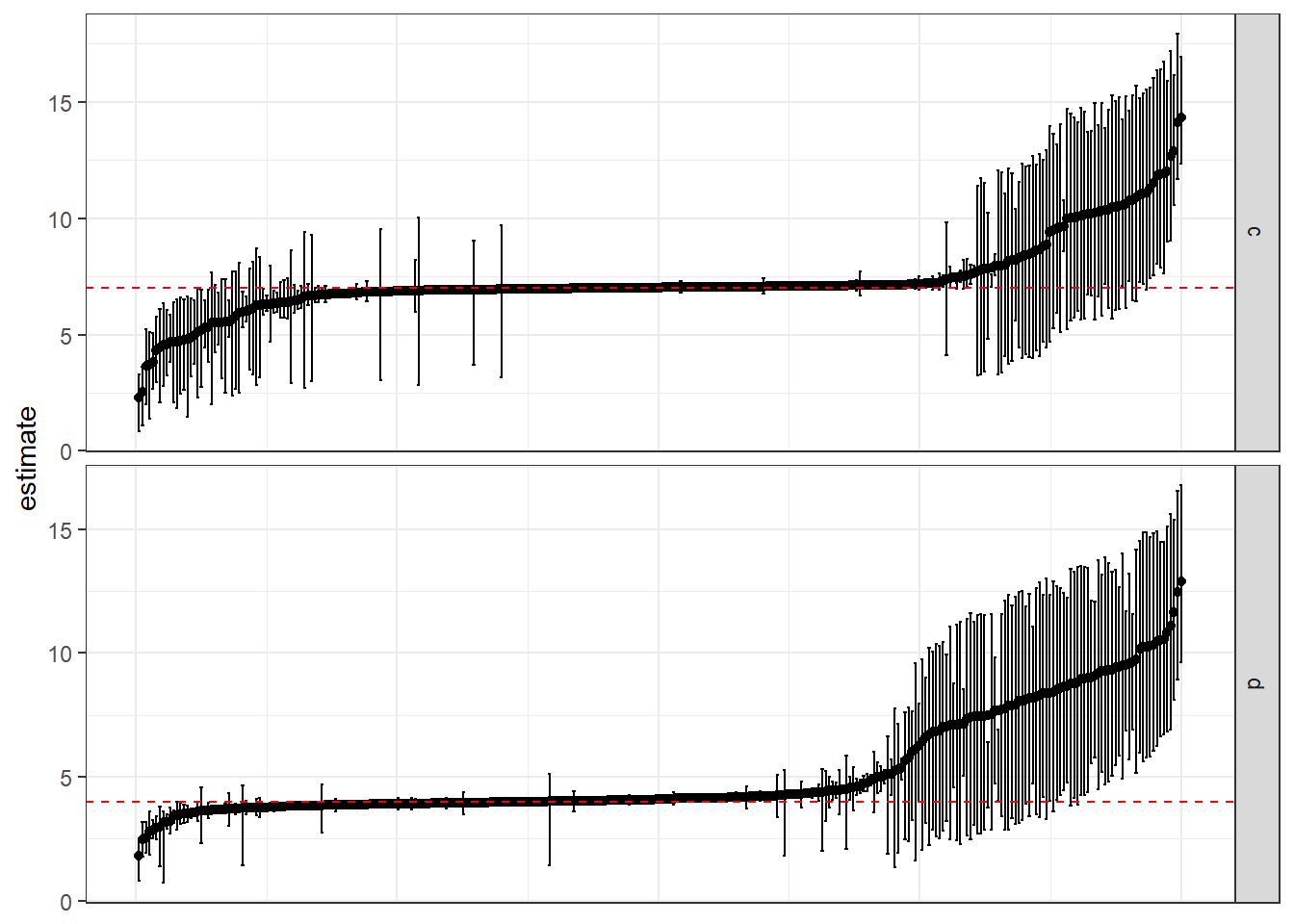
Figure 22.5: Parameter recovery of payoff parameters \(c\) and \(d\), sorted from smallest to greatest. Dots show posterior means, error bars show 50% credible regions (25th-75th percentiles).

To investigate this further, I produced Figure 22.6, which shows just the simulated posterior means as a function of the \(\lambda\) that generated the simulated data. Here we can see that the model is poorly calibrated when \(\lambda\) is very small. This should not be too surprising, because the payoff parameters do not have much bearing on the model’s predictions when \(\lambda\) is small.

dplt<-"Code/HP2024/param_recovery.csv" |>
  read.csv()|>
  filter(parameter=="c" | parameter =="d" | parameter =="lambda") |>
  group_by(simstep) |>
  mutate(lambda.truth = sum(truth*(parameter=="lambda"))) |>
  pivot_wider(
    id_cols = c(simstep,lambda.truth),
    names_from = parameter,
    values_from = mean
  ) |>
  pivot_longer(
    cols = c:d, 
    names_to = "parameter", 
    values_to = "mean"
  )

(
  ggplot(dplt, aes(x=lambda.truth, y=mean))
  +geom_point()
  +facet_grid(parameter~., scales="free")
  +scale_x_continuous(trans = "log10")
  +xlab(expression(lambda~"(true value)"))
  +ylab("posterior mean estimate")
  +theme_bw()
)

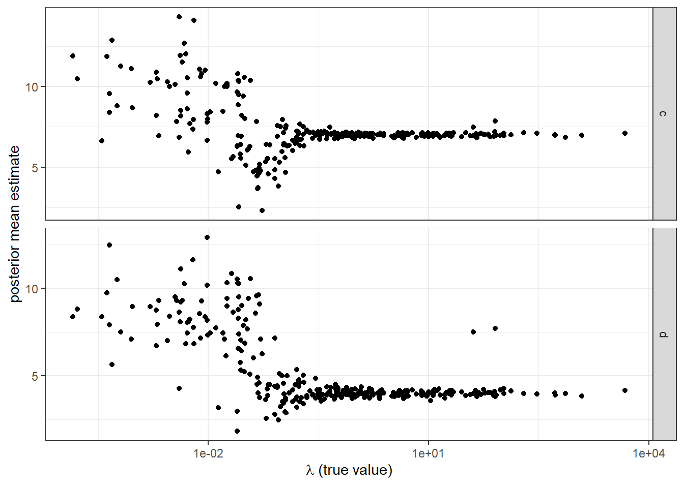
Figure 22.6: Posterior mean estimates from the simulation as a function of the true value of \(\lambda\) (i.e. the value used to simulate the data).

22.4.1.2 Results

Figure 22.7 shows the posterior distributions of \(c\) and \(d\) under different assumptions of logit QRE (solid curves) and Nash equilibrium (dashed curves). Here we can see that both Nash and QRE assumptions do about as well (alternatively: about as badly) at estimating \(d\) (blue curves), but that the QRE model does substantially better at estimating \(c\) (black curves).

Fit<-"Code/HP2024/Fit_QRE_CD_unknown.rds" |>
  readRDS() |>
  as.data.frame()

Fit.Nash<-"Code/HP2024/Fit_Nash_CD_unknown.rds" |>
  readRDS() |>
  as.data.frame()

cd.QRE<-Fit |> 
  dplyr::select(c,d) |>
  pivot_longer(
    cols = c(c,d),
    names_to = "payoff",
    values_to = "value"
  ) |>
  mutate(
    model = "QRE"
  )


cd.Nash<-Fit.Nash |> 
  dplyr::select(c,d) |>
  pivot_longer(
    cols = c(c,d),
    names_to = "payoff",
    values_to = "value"
  ) |>
  mutate(
    model = "Nash"
  )

cd<-rbind(cd.QRE,cd.Nash) |>
  mutate(
    model = model |> factor(levels = c("QRE","Nash"))
  )

(
  ggplot(cd, aes(x=value, color = payoff, linetype=model))
  +geom_density(linewidth=1)
  +scale_color_manual(values = c("black","blue"))
  +theme_bw()
  +geom_hline(yintercept = 0.1, linetype="dashed")
  +xlim(c(0,10))
  +geom_vline(data = data.frame(x = c(7,3),payoff = c("c","d")), aes(xintercept=x, color = payoff))
)

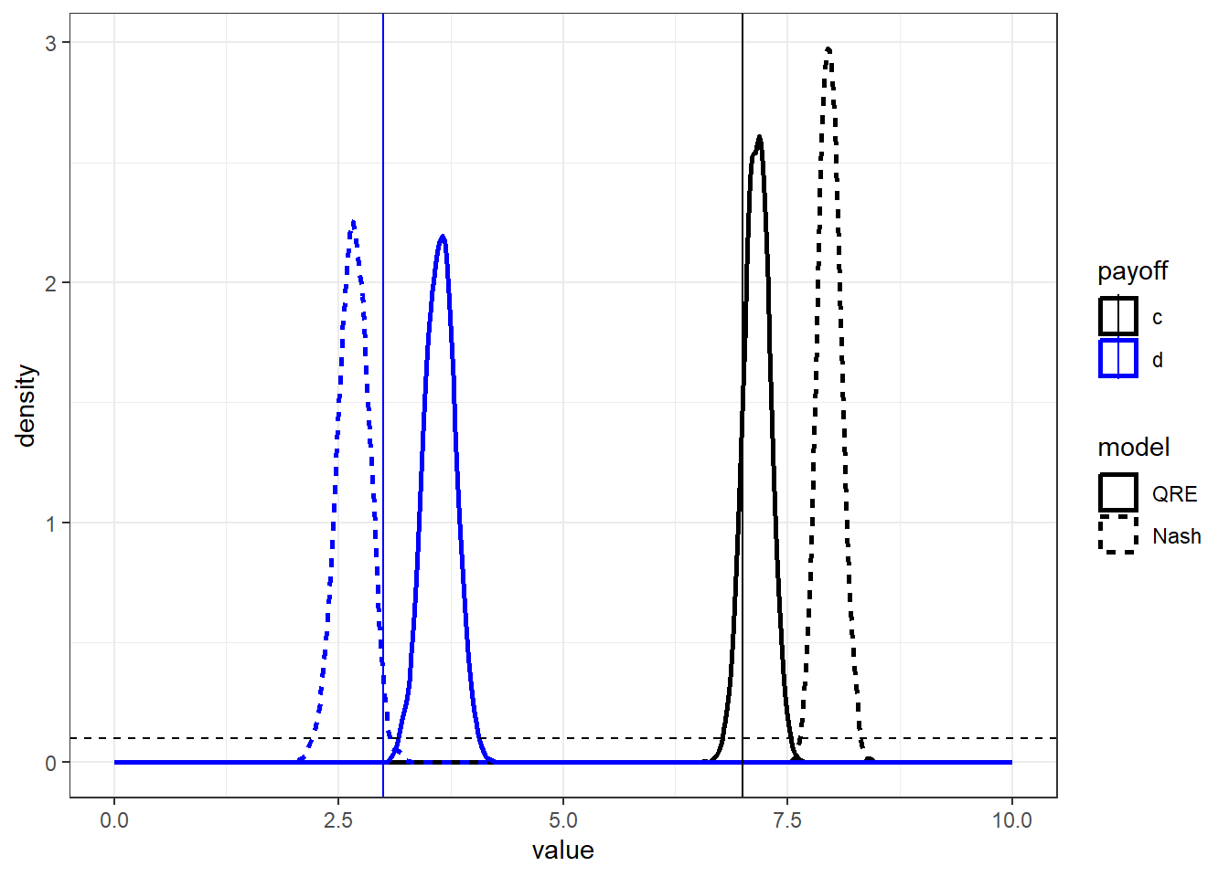
Figure 22.7: Posterior distribution of payoff parameters \(c\) and \(d\).. Vertical dashed lines show true values. Horizontal dashed line shows prior distribution.

But before moving on, we should also have a look at the logit QRE locus, and compare this to the predictions of our QRE model with unknown \(c\) and \(d\) payoff parameters.

locus<-"Code/HP2024/Fit_QRE_CD_unknown.rds" |>
  readRDS() |> 
  as.data.frame() |>
  dplyr::select(lambda, contains("Top"), contains("Left")) |>
  mutate(
    simstep = 1:n()
  ) |>
  pivot_longer(
    cols = `pTop[1]`:`pLeft[4]`,
    names_to = "name",
    values_to = "prob"
  ) |>
  mutate(
    action = ifelse(grepl("Top",name), "Top","Left"),
    treatment.id = name |>  parse_number()
  ) |>
  full_join("Code/HP2024/collapsed_data.csv" |>
              read.csv(),
            by = "treatment.id"
            ) |>
  mutate(
    treatment.txt = paste0("a = ",a,", b = ",b)
  ) |>
  pivot_wider(
    id_cols = c(simstep,lambda, treatment.txt, treatment.id), 
    names_from = action, 
    values_from = prob
  )

(
  ggplot()
  +geom_point(data=locus, aes(x=Top, y=Left, color = treatment.txt), size=0.1, alpha = 0.2)
  +geom_path(data=pc, aes(x=Top, y=Left, color = treatment.txt))
  +geom_text(data=d, aes(x=pTop, y=pLeft,label="X", color=treatment.txt))
  +theme_bw()
  +guides(color = guide_legend(override.aes = list(size = 3, alpha = 1)))
  +scale_color_manual(name = "treatment",values = c("black", "red", "blue"))
)

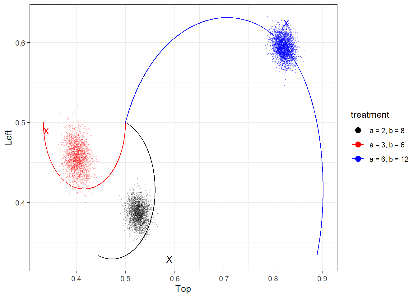
Figure 22.8: Logit QRE locus (curves) assuming known payoff parameters alongside posterior model predictions allowing \(\lambda\), \(c\), and \(d\) to be free parameters (dots). Points marked ‘X’ are treatment-specific empirical choice frequencies.

22.4.2 Unknown \(a\) and \(b\)

Next, I try the harder task of recovering the payoff parameters \(a\) and \(b\). This is harder because these parameters vary by treatment, and so there are eight of them to estimate, rather than two.

Here is the Stan program I wrote to recover \(a\) and \(b\) with the logit QRE model:

functions {
  
  
#include input_QREsolver.stan
  
}

data {
  
  int nTreat; // number of treatments
  
  vector[nTreat] C, D;
  
  array[nTreat] int count, top, left;
  
  int<lower=0, upper=1> UseData;
  
  vector[2] prior_lambda;
  
  int<lower=1> maxiter;
  real<lower=0> tol;
  
  real<lower=0> payoffUB;
  
}


parameters {
  
  vector<lower=0, upper=7>[nTreat] A;
  vector<lower=fmax(A,4), upper=payoffUB>[nTreat] B;
  
  real<lower=0> lambda;
  
}

transformed parameters {
  
  array[nTreat] vector[2] logitp;
  
  vector[nTreat] pTop, pLeft;
  
  for (tt in 1:nTreat) {
    logitp[tt] = lpQRE(
    lambda,
    A[tt],B[tt],C[tt],D[tt],
    maxiter, tol
    );
    
    pTop[tt] = inv_logit(logitp[tt][1]);
    pLeft[tt] = inv_logit(logitp[tt][2]);
  }
  
}


model {
  
  lambda ~ lognormal(prior_lambda[1], prior_lambda[2]);
  
  if (UseData==1) {
    for (tt in 1:nTreat) {
    
      
      top[tt] ~ binomial_logit(count[tt], logitp[tt][1]);
      left[tt] ~ binomial_logit(count[tt], logitp[tt][2]);
    }
  }
  
  
  
}

And here is its Nash counterpart:

functions {
  
  
#include input_QREsolver.stan
  
}

data {
  
  int nTreat; // number of treatments
  
  vector[nTreat] C, D;
  
  array[nTreat] int count, top, left;
  
  int<lower=0, upper=1> UseData;
  
  vector[2] prior_lambda;
  
  int<lower=1> maxiter;
  real<lower=0> tol;
  
  real<lower=0> payoffUB;
  
  real<lower=0> lambda;
  
}


parameters {
  
  vector<lower=0, upper=7>[nTreat] A;
  vector<lower=fmax(A,4), upper=payoffUB>[nTreat] B;
  
}

transformed parameters {
  
  array[nTreat] vector[2] logitp;
  
  vector[nTreat] pTop, pLeft;
  
  for (tt in 1:nTreat) {
    logitp[tt] = lpQRE(
    lambda,
    A[tt],B[tt],C[tt],D[tt],
    maxiter, tol
    );
    
    pTop[tt] = inv_logit(logitp[tt][1]);
    pLeft[tt] = inv_logit(logitp[tt][2]);
  }
  
}


model {
  
  if (UseData==1) {
    for (tt in 1:nTreat) {
    
      
      top[tt] ~ binomial_logit(count[tt], logitp[tt][1]);
      left[tt] ~ binomial_logit(count[tt], logitp[tt][2]);
    }
  }
  
  
  
}

Figure 22.9 shows the posterior distributions of the payoff parameters against their true values. It seems like both models do eith equally badly or equally well, except for the “3 6 prop” treatment, where Nash seems to pin down the correct numbers better, and maybe “6 12 prop”, where the QRE model might have a slight edge in recovering \(b\).

Fit<-"Code/HP2024/Fit_QRE_AB_unknown.rds" |>
  readRDS() |>
  as.data.frame()

Fit.Nash<-"Code/HP2024/Fit_Nash_AB_unknown.rds" |>
  readRDS() |>
  as.data.frame()

ab.QRE<-Fit |> 
  mutate(simstep = 1:n()) |>
  dplyr::select(simstep,`A[1]`:`B[4]`) |>
  pivot_longer(
    cols = c(`A[1]`:`B[4]`),
    names_to = "name",
    values_to = "value"
  ) |>
  mutate(
    payoff = ifelse(grepl("A",name),"a","b"),
    treatment.ind = name |> parse_number()
  ) |>
  mutate(
    truth = ifelse(payoff=="a",d$a[treatment.ind],d$b[treatment.ind]),
    Treatment = d$Treatment[treatment.ind],
    model = "QRE"
  )

ab.Nash<-Fit.Nash |> 
  mutate(simstep = 1:n()) |>
  dplyr::select(simstep,`A[1]`:`B[4]`) |>
  pivot_longer(
    cols = c(`A[1]`:`B[4]`),
    names_to = "name",
    values_to = "value"
  ) |>
  mutate(
    payoff = ifelse(grepl("A",name),"a","b"),
    treatment.ind = name |> parse_number()
  ) |>
  mutate(
    truth = ifelse(payoff=="a",d$a[treatment.ind],d$b[treatment.ind]),
    Treatment = d$Treatment[treatment.ind],
    model = "Nash"
  )

ab <-rbind(ab.QRE, ab.Nash) |>
  mutate(
    model = model |> factor(levels = c("QRE", "Nash"))
  )
  
  
  
(
  ggplot(ab, aes(x=value, color = payoff, linetype=model))
  +geom_density(linewidth=1)
  +facet_wrap(~Treatment)
  +geom_vline(data=ab, aes(xintercept = truth, color=payoff))
  +theme_bw()
  +guides(color = guide_legend(override.aes = list(size = 3, alpha = 1)))
  +scale_color_manual(name = "treatment",values = c("black", "red", "blue","darkgreen"))
)

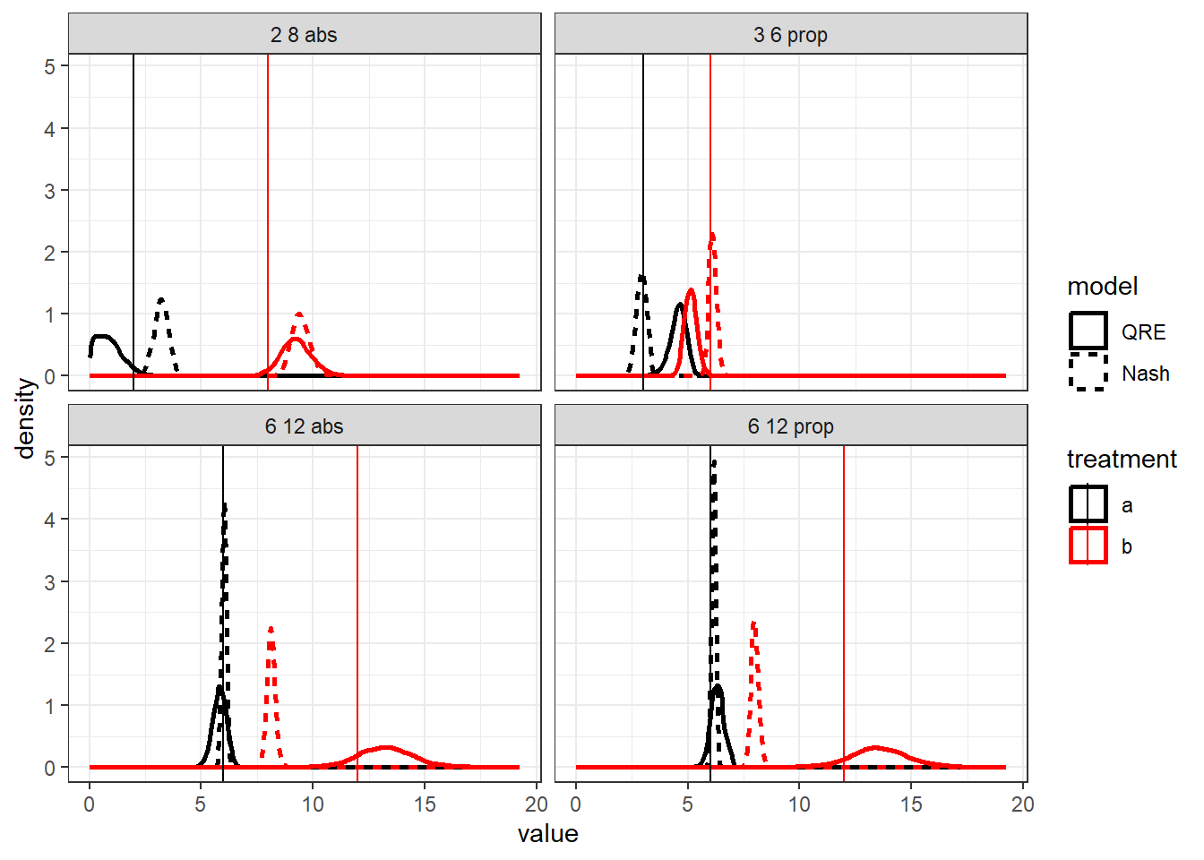
Figure 22.9: Posterior distributions of payoff parameters \(a\) and \(b\) (curves) from the logit QRE model (solid curves) and Nash model (dashed curves). Vertical lines show the true payoff value.

22.5 Heterogeneous pairs

One thing fixed matching does is highlight the heterogeneity between pairs of participants. Case in point Figure 22.10, which shows the empirical choice frequencies for every pair in the experiment. While it is most common for QRE models to ignore this heterogeneity, there are of course extensions to the pooled model that allows us to take the heterogeneity seriously. For this chapter, I will show you how to estimate a hierarchical logit-QRE model where every pair gets their own choice precision, and what I call an “equilibrium in expectation” model.¹⁰³

D<-"Code/HP2024/D_cleaned.csv" |>
  read.csv() |>
  group_by(pairID, Treatment, Role) |>
  summarize(
    pTL = mean(TopLeft)
  ) |>
  pivot_wider(
    id_cols = c(pairID, Treatment),
    names_from = Role,
    values_from = pTL
  ) |>
  mutate(
    treatment.txt = paste0("a = ",Treatment |> str_split_i(" ",1), ", b = ",Treatment |> str_split_i(" ",2))
  ) 



(
  ggplot()
  +geom_jitter(data=D, aes(x=Row, y=Column, color=treatment.txt))
  +geom_path(data=pc, aes(x=Top, y=Left, color = treatment.txt))
  +theme_bw()
  +guides(color = guide_legend(override.aes = list(size = 3, alpha = 1)))
  +scale_color_manual(name = "treatment",values = c("black", "red", "blue"))
  +xlab("Top")
  +ylab("Left")
)

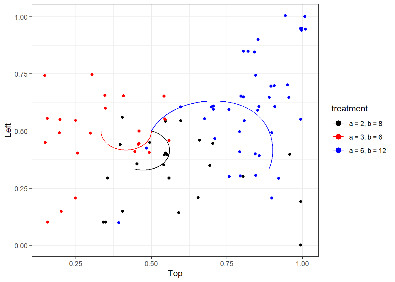
Figure 22.10: Pair-specific empirical choice frequencies (dots) alongside the logit QRE locus (curves). Dots are jittered slightly for clarity.

22.5.1 Hierarchical model

First, we will estimate the hierarchical model. Here, we assume that each pair has their own \(\lambda_i\), which are independent draws from the population distribution. For this, I just assumed a log-normal specification:

\[ \begin{aligned} \lambda_i&\sim \mathrm{lognormal}(\mu_\lambda, \sigma^2_\lambda) \end{aligned} \]

Importantly here while pairs are heterogeneous, they are still forced to play mixed strategies that lie on the logit QRE locus. This will be different with the equilibrium in expectation model.

Here is the code for the hierarchical model. While a lot of it looks the same as the pooled model, the big difference, other than the hierarchical specification, is that we now have to pass data at the pair level to Stan, rather than at the treatment level. Therefore there is a lot more QRE-computing to be done. Also, have a look at the generated quantities block, where I generate pTop_pop and pLeft_pop. These are the predictions of the choice probabilities for a randomly selected new subject (i.e. someone who did not participate in the experiment).

functions {
  
  
  #include input_QREsolver.stan
  
}

data {
  
  int N; // number of obsrevations (pair-treatment pairs)
  array[N] int count, top, left, pairID;
  vector[N] A, B, C, D;
  
  
  int<lower=0, upper=1> UseData;
  
  vector[2] prior_lambda_med;
  real<lower = 0> prior_lambda_sd;
  
  int<lower=1> maxiter;
  real<lower=0> tol;
  
  
  // some things to get the population averaged-predictions
  int nsim;
  vector[nsim] zsim;
  int ntreat;
  vector[ntreat] Atreat, Btreat, Ctreat, Dtreat;
  
}

transformed data {
  
  int nPairs = max(pairID);
  
}


parameters {
  
  real<lower=0> lambda_med;
  real<lower=0> lambda_sd;
  
  vector[nPairs] z; // non-centered parameterization of lambda
  
}

transformed parameters {
  
  vector[nPairs] lambda = exp(log(lambda_med)+lambda_sd*z);
  
  array[N] vector[2] logitp;
  
  vector[N] pTop, pLeft;
  
  for (tt in 1:N) {
    logitp[tt] = lpQRE(
    lambda[pairID[tt]],
    A[tt],B[tt],C[tt],D[tt],
    maxiter, tol
    );
    
    pTop[tt] = inv_logit(logitp[tt][1]);
    pLeft[tt] = inv_logit(logitp[tt][2]);
  }
  
}


model {
  
  lambda_med ~ lognormal(prior_lambda_med[1], prior_lambda_med[2]);
  lambda_sd ~ normal(0.0, prior_lambda_sd);
  
  z ~ std_normal();
  
  
  if (UseData==1) {
    for (tt in 1:N) {
    
      
      top[tt] ~ binomial_logit(count[tt], logitp[tt][1]);
      left[tt] ~ binomial_logit(count[tt], logitp[tt][2]);
    }
  }
  
  
  
}

generated quantities {
  
  vector[ntreat] pTop_pop, pLeft_pop;
  
  for (tt in 1:ntreat) {
    real a = Atreat[tt];
    real b = Btreat[tt];
    real c = Ctreat[tt];
    real d = Dtreat[tt];
    
    vector[nsim] pTop_temp;
    vector[nsim] pLeft_temp;
    
    for (ss in 1:nsim) {
      real l = exp(log(lambda_med)+zsim[ss]*lambda_sd);
      
      vector[2] lp = lpQRE(l,a,b,c,d,maxiter, tol);
      
      pTop_temp[ss] = inv_logit(lp[1]);
      pLeft_temp[ss] = inv_logit(lp[2]);
      
    }
    
    pTop_pop[tt] = mean(pTop_temp);
    pLeft_pop[tt] = mean(pLeft_temp);
    
  }
  
  
  
  
}

Now we can have a look at the hierarchical model’s predictions, which are shown in Figure 22.11. First, we can look at the model’s population-level predictions. The small dots show the posterior draws for this quantity. Importantly here, while the model’s prediction for an individual pair will always be on the locus (solid curves), averaging over these predictions means that the overall prediction will in general not be on the locus (because of Jensen’s inequality). The faint line segments connect the empirical choice frequencies (dots in Figure 22.10) to their matched point on the locus, just using the posterior mean prediction. These can be thought of as the “shrinkage” estimates of the pairs’ predictions. Again, while each posterior draw of the pairs’ predictions will lie on the locus, the means of these will not because of Jensen’s inequality.

Fit<-"Code/HP2024/Fit_QRE_known_parameters_hierarchical.rds" |>
  readRDS()

Fit.df <- Fit |>
  as.data.frame() |>
  mutate(
    simstep = 1:n()
  )

pair.means<-summary(Fit)$summary |>
  data.frame() |>
  rownames_to_column(var = "par") |>
  filter(
    (grepl("pTop", par) | grepl("pLeft", par)) & !grepl("_pop", par)
  ) |>
  mutate(
    action = ifelse(grepl("pTop", par), "pTop", "pLeft"),
    pair.id = par |> parse_number()
  ) |>
  pivot_wider(
    id_cols = pair.id,
    names_from = action,
    values_from = mean
  ) 
  

pop<-Fit.df |>
  dplyr::select(simstep,contains("_pop")) |>
  pivot_longer(
    cols = `pTop_pop[1]`:`pLeft_pop[4]`,
    names_to = "name",
    values_to = "value"
  ) |>
  mutate(
    treatment.id = name |> parse_number(),
    action = ifelse(grepl("pTop",name),"Top","Left")
  )  |>
  pivot_wider(
    id_cols = c(simstep, treatment.id),
    names_from = action,
    values_from = value
  ) |>
  full_join("Code/HP2024/collapsed_data.csv" |>
              read.csv(),
            by = "treatment.id"
            ) |>
  mutate(
    treatment.txt = paste0("a = ",a,", b = ",b)
  )

pair.means<-cbind(pair.means,D)

(
  ggplot()
  +geom_segment(data=pair.means, aes(x=pTop, y=pLeft, xend = Row, yend = Column, color = treatment.txt), alpha = 0.2)
  +geom_point(data=pop, aes(x=Top, y=Left, color = treatment.txt), size=0.1, alpha = 0.1)
  +geom_path(data=pc, aes(x=Top, y=Left, color = treatment.txt))
  +guides(color = guide_legend(override.aes = list(size = 3, alpha = 1)))
  +scale_color_manual(name = "treatment",values = c("black", "red", "blue"))
   +theme_bw()
  +xlab("Top")+ylab("Left")
)

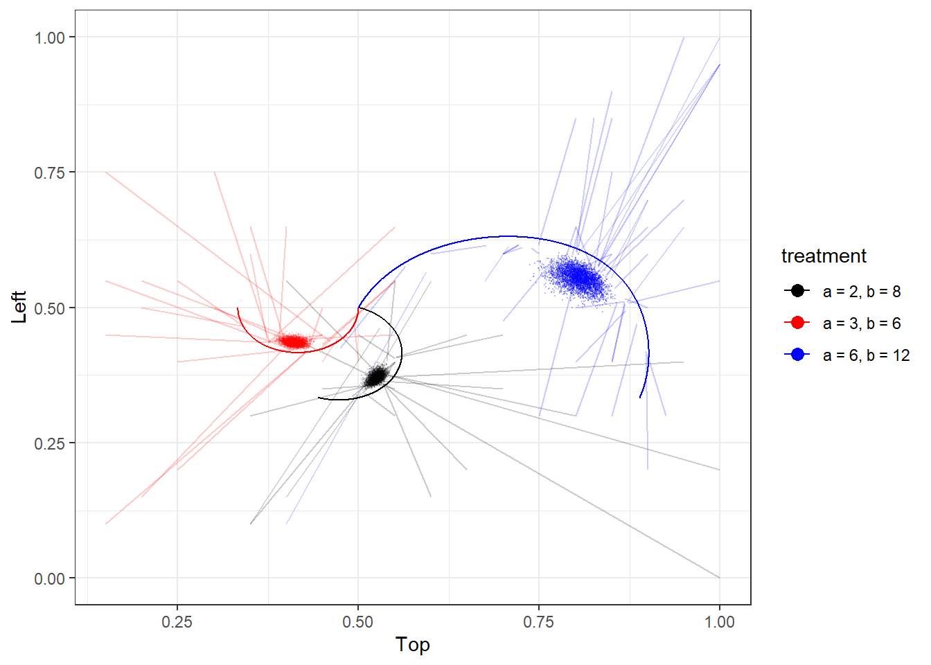
Figure 22.11: Visualization of the hierarchical model. Solid curves show the logit QRE locus. Dots show posterior draws from the model’s mean prediction. Faint line segments connect data (a pair’s empirical choice frequency) with their point on the locus.

22.5.2 Equilibrium in expectation model

Finally, we turn to a model that does not take the logit QRE locus so seriously. This is the “equilibrium in expectation” model, which I developed for Bland (2026). Here we assume that each pair \(i\) plays mixed strategies \(\{q_i^\mathrm{Top}, q_i^\mathrm{Left}\}\), which do not have to be on the locus. But in the population, these mixed strategies are centered on the locus. That is, the model has the following hierarchical structure:

\[ \begin{aligned} q_i^\mathrm{Top}&\sim \mathrm{Beta}\left(\kappa p^\mathrm{Top}(\lambda), \kappa (1-p^\mathrm{Top}(\lambda))\right)\\ q_i^\mathrm{Left}&\sim \mathrm{Beta}\left(\kappa p^\mathrm{Left}(\lambda), \kappa (1-p^\mathrm{Left}(\lambda))\right) \end{aligned} \]

That is, \(\kappa>0\) is the new parameter, which measures the concentration of mixed strategies around the point on the QRE locus. We can therefore use this to measure how closely participants are playing to the logit QRE locs. Here I use the Beta distribution (rather than, say logit-normal or probit-normal), because the Beta preserves the expectation, as in \(E[q_i^X\mid \lambda]=p^X\). Hence the name of the model.

Here is the Stan program for estimating the equilibrium in expectation model.

functions {
  
  
  #include input_QREsolver.stan
  
}

data {
  
  int N; // number of obsrevations (pair-treatment pairs)
  array[N] int count, top, left, pairID;
  vector[N] A, B, C, D;
  
  
  int<lower=0, upper=1> UseData;
  
  vector[2] prior_lambda;
  real<lower=0> prior_kappa;
  
  int<lower=1> maxiter;
  real<lower=0> tol;
  
  
  // some things to get the population averaged-predictions
  int nsim;
  vector[nsim] zsim;
  int ntreat;
  vector[ntreat] Atreat, Btreat, Ctreat, Dtreat;
  
}

transformed data {
  
  int nPairs = max(pairID);
  
}


parameters {
  
  real<lower=0> lambda;
  
  real<lower=0> kappa;
  
  vector<lower=0, upper=1>[N] pTop_g, pLeft_g;
  
  
}



transformed parameters {
  
  array[N] vector[2] logitp;
  
  vector[N] pTop, pLeft;
  
  for (tt in 1:N) {
    logitp[tt] = lpQRE(
    lambda,
    A[tt],B[tt],C[tt],D[tt],
    maxiter, tol
    );
    
    pTop[tt] = inv_logit(logitp[tt][1]);
    pLeft[tt] = inv_logit(logitp[tt][2]);
  }
  
}


model {
  
  lambda ~ lognormal(prior_lambda[1], prior_lambda[2]);
  kappa ~ normal(0.0, prior_kappa);
  
  
  pTop_g ~ beta(kappa*pTop, kappa*(1.0-pTop));
  pLeft_g ~ beta(kappa*pLeft, kappa*(1.0-pLeft));
  
  if (UseData==1) {
    
    top ~ binomial(count, pTop_g);
    left ~ binomial(count, pLeft_g);
    
  }
  
  
  
}

generated quantities {
  
  vector[ntreat] pTop_pop, pLeft_pop;
  
  for (tt in 1:ntreat) {
    real a = Atreat[tt];
    real b = Btreat[tt];
    real c = Ctreat[tt];
    real d = Dtreat[tt];
    
    vector[nsim] pTop_temp;
    vector[nsim] pLeft_temp;
    
    for (ss in 1:nsim) {
      
      vector[2] lp = lpQRE(lambda,a,b,c,d,maxiter, tol);
      
      pTop_temp[ss] = inv_logit(lp[1]);
      pLeft_temp[ss] = inv_logit(lp[2]);
      
    }
    
    pTop_pop[tt] = mean(pTop_temp);
    pLeft_pop[tt] = mean(pLeft_temp);
    
  }
  
  
  
  
}

Figure 22.12 visualizes the posterior distribution of this model. Here we can see that the model’s predictions (small dots) are all on the QRE locus (unlike the hierarchical model). The pair-specific choice frequencies are denoted with an \(X\), and are connected by line segments to their corresponding mixes strategy shrinkage estimates. Here we can see that there is a lot of off-equilibrium behavior, with most line segments not coming close to their corresponding locus.

Fit<-"Code/HP2024/Fit_QRE_known_parameters_eqexp.rds" |>
  readRDS()

Fit.df <- Fit |>
  as.data.frame() |>
  mutate(
    simstep = 1:n()
  )

pair.means<-summary(Fit)$summary |>
  data.frame() |>
  rownames_to_column(var = "par") |>
  filter(
    (grepl("pTop_g", par) | grepl("pLeft_g", par)) 
  ) |>
  mutate(
    action = ifelse(grepl("pTop", par), "pTop", "pLeft"),
    pair.id = par |> parse_number()
  ) |>
  pivot_wider(
    id_cols = pair.id,
    names_from = action,
    values_from = mean
  ) 
  

pop<-Fit.df |>
  dplyr::select(simstep,contains("_pop")) |>
  pivot_longer(
    cols = `pTop_pop[1]`:`pLeft_pop[4]`,
    names_to = "name",
    values_to = "value"
  ) |>
  mutate(
    treatment.id = name |> parse_number(),
    action = ifelse(grepl("pTop",name),"Top","Left")
  )  |>
  pivot_wider(
    id_cols = c(simstep, treatment.id),
    names_from = action,
    values_from = value
  ) |>
  full_join("Code/HP2024/collapsed_data.csv" |>
              read.csv(),
            by = "treatment.id"
            ) |>
  mutate(
    treatment.txt = paste0("a = ",a,", b = ",b)
  )

pair.means<-cbind(pair.means,D)

(
  ggplot()
  +geom_segment(data=pair.means, aes(x=pTop, y=pLeft, xend = Row, yend = Column, color = treatment.txt), alpha = 0.2)
  +geom_text(data=pair.means, aes(x = Row, y = Column, color = treatment.txt, label="X"), alpha = 0.2)
  +geom_jitter(data=pop, aes(x=Top, y=Left, color = treatment.txt), size=0.1, alpha = 0.1,
               width=0.01, height=0.01
               )
  +geom_path(data=pc, aes(x=Top, y=Left, color = treatment.txt))
  +guides(color = guide_legend(override.aes = list(size = 3, alpha = 1)))
  +scale_color_manual(name = "treatment",values = c("black", "red", "blue"))
   +theme_bw()
  +xlab("Top")+ylab("Left")
)

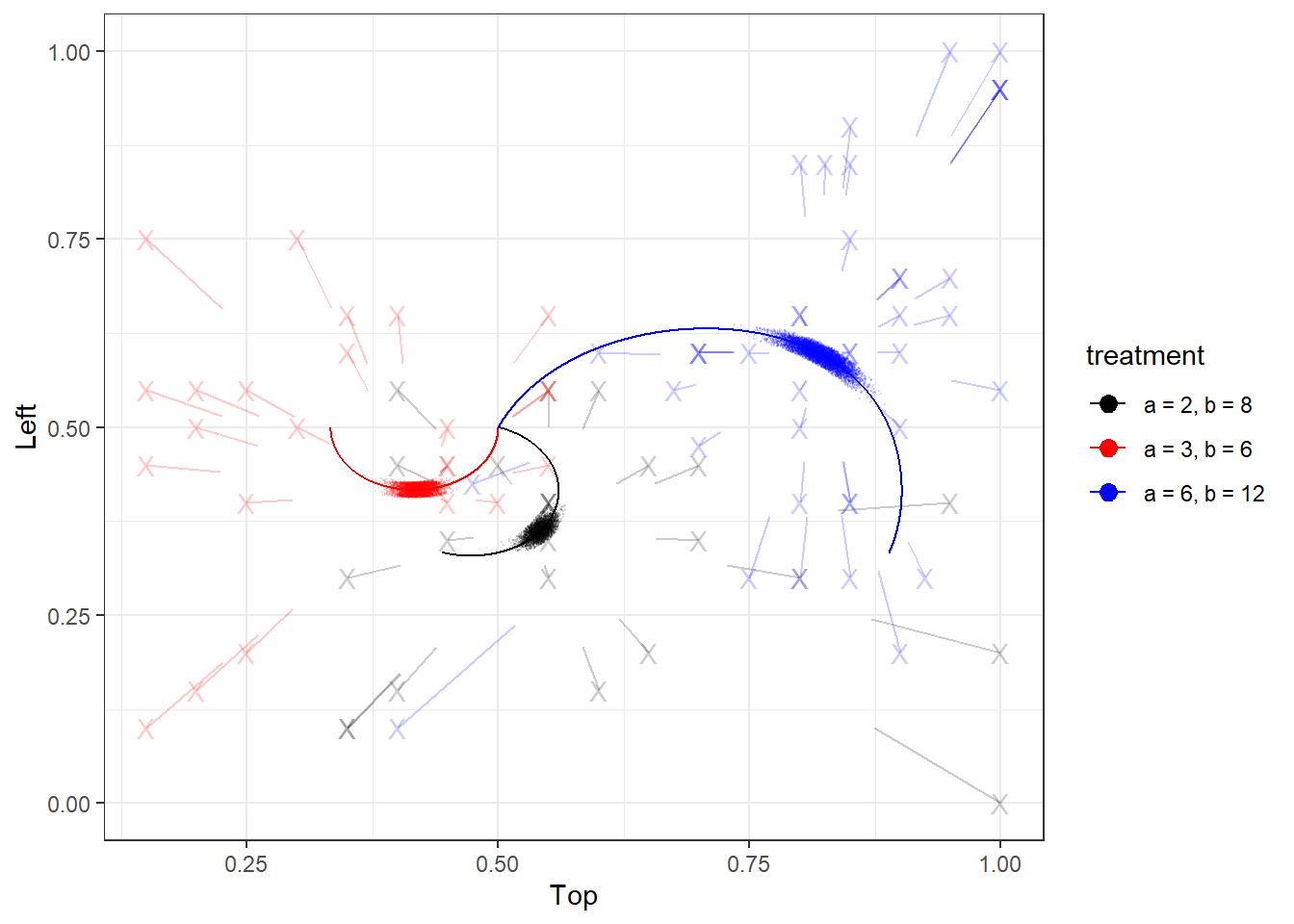
Figure 22.12: Visualization of the equilibrium in expectation model. Solid curves show the logit QRE locus. Dots show posterior draws from the model’s mean prediction (jittered for clarity). Faint line segments connect data (a pair’s empirical choice frequency, also denoted with an ‘X’) with their estimated mixed strategy.

To finish with, how can we interpret the new parameter \(\kappa\), which measures concentration around the QRE locus? This is particularly difficult because \(\kappa\to\infty\) corresponds to all play being exactly on the locus. To try to answer this, I note that the standard deviation of the Beta distribution is greatest when its mean is \(0.5\), in which case it becomes:

\[ \frac{0.5}{\sqrt{\kappa+1}} \]

so let’s work with this quantity. Figure 22.13 shows the posterior and prior distributions of this quantity, with the posterior shown with the solid curve. Here we can see that there is substantial updating between the prior and posterior, and that most of the posterior mass is around \(0.15\). For a variable that is bounded between zero and one, this is quite a substantial value. Therefore we can conclude that off-equilibrium play at the pair level is substantial.

set.seed(42)

d<-Fit.df |>
  dplyr::select(kappa) |>
  mutate(
    posterior = 0.5/sqrt(kappa+1),
    kappa.prior = rnorm(n(),mean=0, sd=5) |> abs(),
    prior = 0.5/sqrt(kappa.prior+1)
  ) |>
  pivot_longer(
    cols = c(posterior, prior),
    names_to = "distribution", 
    values_to = "value"
  )

(
  ggplot(d, aes(x=value, linetype=distribution))
  +geom_density(linewidth=1)
  +theme_bw()
  +xlab(expression("maximum sd = 0.5/("*kappa*"+1)"))
)

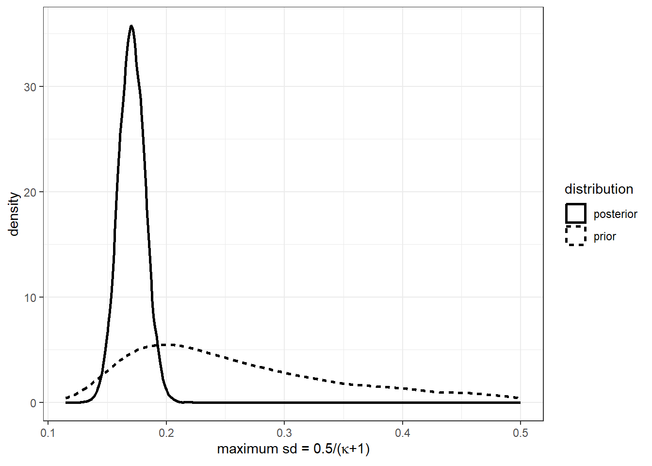
Figure 22.13: Distribution of the maximum possible standard deviation implied by concentration parameter \(\kappa\).

R code used for this chapter

library(tidyverse)
library(rstan)
options(mc.cores = parallel::detectCores())
rstan_options(auto_write = TRUE)
library(readxl)

D<-"Data/HP2024/All_Data.xlsx" |>
  read_excel() |>
  mutate(
    Role = ifelse(`Role (1=row, 2=col_attacker)`==1, "Row", "Column"),
    # See note on p4 of README_replication_file.pdf:
    # Note: the payoff matrix for the Veconlab setup has the columns in different 
    # order from the order listed in the payoff matrix in the paper itself. This c
    # hange was done so that the figures with best response lines did not form a 
    # “sqastika” pattern. Thus the right column (coded as attack 2 in the excel 
    #sheet is “attack 1” in the paper, so the data counts will count the number 
    # of own Decision that are “2” in order to calculate the attack 1 frequency 
    # by round used in figure 6.
    # But I also suspect this is the case for the row player as well
    TopLeft = ifelse(`Decision (1=Top,1=Left)`==2,1,0),
    id.role = ifelse(Role=="Row", ID, `Other ID`),
    arm = ifelse(`Treatment Arm  (1=prop, 2=abs)`==1,"prop","abs"),
    pairID = paste(Session,"-",id.role)
  ) 

D |>
  write_csv("Code/HP2024/D_cleaned.csv")



#-------------------------------------------------------------------------------
# My attempt to replicate Figure 5
#-------------------------------------------------------------------------------

dplt<-D |>
  filter(
    arm == "abs"
  ) |>
  group_by(
    Treatment, Round, Role
  ) |>
  summarize(
    TopLeft = mean(TopLeft)
  ) |>
  pivot_wider(
    id_cols = c(Treatment,Round),
    names_from = Role,
    values_from = TopLeft
  ) 

(
  ggplot(dplt, aes(x=Round, y=Column, color = Treatment, group=paste(Round>20, Treatment)))
  +geom_line(linewidth=1)
  +geom_vline(xintercept = 20.5)
  +geom_hline(yintercept=1/3, linetype="dashed")
  +theme_bw()
  +scale_color_manual(values = c("red","blue"))
)


# looks good



# estimation data

d<-D |>
  #filter(Round>21) |>
  mutate(
    Treatment = paste(Treatment, ifelse(`Treatment Arm  (1=prop, 2=abs)`==1,"prop","abs"))
  ) |>
  pivot_wider(
    id_cols = c(Session, Treatment, Round, id.role),
    names_from = Role,
    values_from = TopLeft
  ) |>
  group_by(Treatment) |>
  summarize(
    top = sum(Row),
    left = sum(Column),
    count = n(),
    nsubj.player1 = length(unique(paste(id.role,Session)))
  ) |>
  mutate(
    a = Treatment |> str_split_i(" ", 1) |> as.numeric(),
    b = Treatment |> str_split_i(" ", 2) |> as.numeric(),
    treatment.id = 1:n()
  )

d |>
  write.csv("Code/HP2024/collapsed_data.csv")

model.known.parameters <- "Code/HP2024/QRE_known_parameters.stan" |>
  stan_model()

#-------------------------------------------------------------------------------
# Prior check
#-------------------------------------------------------------------------------

file<-"Code/HP2024/lambda_prior_check.csv"

if (!file.exists(file)) {
  
  priorcheck<-data.frame()
  
  for (lambda.sd in c(1,3,9,27)) {
    
    print(lambda.sd)
    
    dStan<-list(
      nTreat = dim(d)[1],
      A = d$a,
      B = d$b,
      C = rep(7,dim(d)[1]),
      D = rep(4, dim(d)[1]),
      count = d$count,
      top = d$top,
      left = d$left,
      
      UseData = 0,
      
      prior_lambda = c(log(0.3), lambda.sd),
      
      maxiter = 100,
      tol = 1e-4
    )
    
    PRIOR<-model.known.parameters |>
      sampling(data=dStan,
               seed=42)
    
    priorcheck<-rbind(priorcheck,
                      PRIOR |>
                        as.data.frame() |>
                        mutate(
                          lambda.sd = lambda.sd,
                          simstep = 1:n()
                        )
    )
    
  }
  
  priorcheck |> write.csv(file)
  
}

#-------------------------------------------------------------------------------
# Estimation with known parameters
#-------------------------------------------------------------------------------

file<-"Code/HP2024/Fit_QRE_known_parameters.rds"

if (!file.exists(file)) {
  
  
  dStan<-list(
    nTreat = dim(d)[1],
    A = d$a,
    B = d$b,
    C = rep(7,dim(d)[1]),
    D = rep(4, dim(d)[1]),
    count = d$count,
    top = d$top,
    left = d$left,
    
    UseData = 1,
    
    prior_lambda = c(log(0.3), 3),
    
    maxiter = 100,
    tol = 1e-4
  )
  
  Fit<-model.known.parameters |>
    sampling(data=dStan,
             seed=42
    )
  
  Fit |>
    saveRDS(file)
}

#-------------------------------------------------------------------------------
# Unknown lambda, c, and d
#-------------------------------------------------------------------------------

file<-"Code/HP2024/Fit_QRE_CD_unknown.rds"

if (!file.exists(file) ) {
  
  model.unknown.CD <- "Code/HP2024/QRE_CD_unknown.stan" |>
    stan_model()
  
  
  dStan<-list(
    nTreat = dim(d)[1],
    A = d$a,
    B = d$b,
    count = d$count,
    top = d$top,
    left = d$left,
    
    UseData = 1,
    
    prior_lambda = c(log(0.3), 3),
    
    maxiter = 100,
    tol = 1e-4,
    payoffUB = 20
  )
  
  Fit<-model.unknown.CD |>
    sampling(data=dStan,
             seed=42
    )
  
  Fit |>
    saveRDS(file)
}


#-------------------------------------------------------------------------------
# Unknown, c, and d, Nash
#-------------------------------------------------------------------------------

file<-"Code/HP2024/Fit_Nash_CD_unknown.rds"

if (!file.exists(file)) {
  
  model.unknown.CD <- "Code/HP2024/Nash_CD_unknown.stan" |>
    stan_model()
  
  
  dStan<-list(
    nTreat = dim(d)[1],
    A = d$a,
    B = d$b,
    count = d$count,
    top = d$top,
    left = d$left,
    
    UseData = 1,
    
    prior_lambda = c(log(0.3), 3),
    
    maxiter = 100,
    tol = 1e-4,
    payoffUB = 20,
    
    lambda = 1000
  )
  
  Fit<-model.unknown.CD |>
    sampling(data=dStan,
             seed=42
    )
  
  Fit |>
    saveRDS(file)
}

#-------------------------------------------------------------------------------
# Unknown, a, and b, Nash
#-------------------------------------------------------------------------------

file<-"Code/HP2024/Fit_Nash_AB_unknown.rds"

if (!file.exists(file)) {
  
  model.unknown.AB <- "Code/HP2024/Nash_AB_unknown.stan" |>
    stan_model()
  
  
  dStan<-list(
    nTreat = dim(d)[1],
    C = rep(7,4),
    D = rep(4,4),
    count = d$count,
    top = d$top,
    left = d$left,
    
    UseData = 1,
    
    prior_lambda = c(log(0.3), 3),
    
    maxiter = 100,
    tol = 1e-4,
    payoffUB = 20,
    
    lambda = 1000
  )
  
  Fit<-model.unknown.AB |>
    sampling(data=dStan,
             seed=42
    )
  
  Fit |>
    saveRDS(file)
}




#-------------------------------------------------------------------------------
# Unknown lambda, a, and b
#-------------------------------------------------------------------------------

file<-"Code/HP2024/Fit_QRE_AB_unknown.rds"

if (!file.exists(file)) {
  
  model.unknown.AB <- "Code/HP2024/QRE_AB_unknown.stan" |>
    stan_model()
  
  
  dStan<-list(
    nTreat = dim(d)[1],
    C = rep(7,dim(d)[1]),
    D = rep(4, dim(d)[1]),
    count = d$count,
    top = d$top,
    left = d$left,
    
    UseData = 1,
    
    prior_lambda = c(log(0.3), 3),
    
    maxiter = 100,
    tol = 1e-4,
    payoffUB = 20
  )
  
  Fit<-model.unknown.AB |>
    sampling(data=dStan,
             seed=42
    )
  
  Fit |>
    saveRDS(file)
}


#-------------------------------------------------------------------------------
# Hierarchical, known parameters
#-------------------------------------------------------------------------------

file<-"Code/HP2024/Fit_QRE_known_parameters_hierarchical.rds"

if (!file.exists(file)) {

  dh<-D |>
    group_by(pairID,Treatment, Role) |>
    summarize(
      TL = sum(TopLeft),
      count = n()
    ) |>
    pivot_wider(
      id_cols = c(pairID, Treatment, count),
      names_from = Role,
      values_from = TL
    ) |>
    mutate(
      pairID = as.factor(pairID),
      a = Treatment |> str_split_i(" ",1) |> as.numeric(),
      b = Treatment |> str_split_i(" ",2) |> as.numeric()
    )
  
  model.hierarchical<-"Code/HP2024/QRE_known_parameters_hierarchical.stan" |>
    stan_model()
  
  set.seed(67)
  
  dStan<-list(
    N = dim(dh)[1],
    count = dh$count,
    top = dh$Row,
    left = dh$Column,
    pairID = dh$pairID |> as.numeric(),
    
    A = dh$a,
    B = dh$b, 
    C = rep(7, dim(dh)[1]),
    D = rep(4, dim(dh)[1]),
    
    UseData = 1,
    
    prior_lambda_med = c(log(0.3), 3),
    prior_lambda_sd = 5,
    
    maxiter = 100,
    tol = 1e-4,
    
    nsim = 1000,
    zsim = rnorm(1000),
    ntreat = dim(d)[1],
    Atreat = d$a,
    Btreat = d$b,
    Ctreat = rep(7,4),
    Dtreat = rep(4,4)
  )
  
  Fit<-model.hierarchical |>
    sampling(
      data=dStan,
      pars = c("z","logitp"), include=FALSE,
      seed=42
    )
  
  Fit |>
    saveRDS(file)
  
  
}
  


#-------------------------------------------------------------------------------
# Hierarchical, unknown C & D
#-------------------------------------------------------------------------------

file<-"Code/HP2024/Fit_QRE_CD_unknown_hierarchical.rds"

if (!file.exists(file)) {
  
  dh<-D |>
    group_by(pairID,Treatment, Role) |>
    summarize(
      TL = sum(TopLeft),
      count = n()
    ) |>
    pivot_wider(
      id_cols = c(pairID, Treatment, count),
      names_from = Role,
      values_from = TL
    ) |>
    mutate(
      pairID = as.factor(pairID),
      a = Treatment |> str_split_i(" ",1) |> as.numeric(),
      b = Treatment |> str_split_i(" ",2) |> as.numeric()
    )
  
  model.hierarchical<-"Code/HP2024/QRE_CD_unknown_hierarchical.stan" |>
    stan_model()
  
  set.seed(67)
  
  dStan<-list(
    N = dim(dh)[1],
    count = dh$count,
    top = dh$Row,
    left = dh$Column,
    pairID = dh$pairID |> as.numeric(),
    
    A = dh$a,
    B = dh$b, 
    C = rep(7, dim(dh)[1]),
    D = rep(4, dim(dh)[1]),
    
    UseData = 1,
    
    prior_lambda_med = c(log(0.3), 3),
    prior_lambda_sd = 5,
    
    maxiter = 100,
    tol = 1e-4,
    
    nsim = 1000,
    zsim = rnorm(1000),
    ntreat = dim(d)[1],
    Atreat = d$a,
    Btreat = d$b,
    
    payoffUB = 20
    
  )
  
  Fit<-model.hierarchical |>
    sampling(
      data=dStan,
      pars = c("z","logitp"), include=FALSE,
      seed=42
    )
  
  Fit |>
    saveRDS(file)
  
  
}


#-------------------------------------------------------------------------------
# Hierarchical, unknown A & B
#-------------------------------------------------------------------------------

file<-"Code/HP2024/Fit_QRE_AB_unknown_hierarchical.rds"

if (!file.exists(file) ) {
  
  dh<-D |>
    group_by(pairID,Treatment, Role,arm) |>
    summarize(
      TL = sum(TopLeft),
      count = n()
    ) |>
    pivot_wider(
      id_cols = c(pairID, Treatment, count,arm),
      names_from = Role,
      values_from = TL
    ) |>
    mutate(
      pairID = as.factor(pairID),
      a = Treatment |> str_split_i(" ",1) |> as.numeric(),
      b = Treatment |> str_split_i(" ",2) |> as.numeric(),
      Treatment = paste(Treatment, arm)
    ) |>
    full_join(
      d |> select(Treatment, treatment.id) ,
      by = "Treatment"
    )
  
  model.hierarchical<-"Code/HP2024/QRE_AB_unknown_hierarchical.stan" |>
    stan_model()
  
  set.seed(67)
  
  dStan<-list(
    N = dim(dh)[1],
    count = dh$count,
    top = dh$Row,
    left = dh$Column,
    pairID = dh$pairID |> as.numeric(),
    treatID = dh$treatment.id,
    
    c = 7,
    d = 4,
    
    UseData = 1,
    
    prior_lambda_med = c(log(0.3), 3),
    prior_lambda_sd = 5,
    
    maxiter = 100,
    tol = 1e-4,
    
    nsim = 1000,
    zsim = rnorm(1000),
    ntreat = dim(d)[1],
    
    
    payoffUB = 20
    
  )
  
  Fit<-model.hierarchical |>
    sampling(
      data=dStan,
      # running into some ESS issues
      iter = 4000, chains = 8,
      pars = c("z","logitp"), include=FALSE,
      seed=42
    )
  
  Fit |>
    saveRDS(file)
  
  
}

#-------------------------------------------------------------------------------
# Equilibrium in expectation,  known parameters
#-------------------------------------------------------------------------------

file<-"Code/HP2024/Fit_QRE_known_parameters_eqexp.rds"

if (!file.exists(file)) {
  
  dh<-D |>
    group_by(pairID,Treatment, Role) |>
    summarize(
      TL = sum(TopLeft),
      count = n()
    ) |>
    pivot_wider(
      id_cols = c(pairID, Treatment, count),
      names_from = Role,
      values_from = TL
    ) |>
    mutate(
      pairID = as.factor(pairID),
      a = Treatment |> str_split_i(" ",1) |> as.numeric(),
      b = Treatment |> str_split_i(" ",2) |> as.numeric()
    )
  
  model.eqexp<-"Code/HP2024/QRE_known_parameters_eqexp.stan" |>
    stan_model()
  
  set.seed(67)
  
  dStan<-list(
    N = dim(dh)[1],
    count = dh$count,
    top = dh$Row,
    left = dh$Column,
    pairID = dh$pairID |> as.numeric(),
    
    A = dh$a,
    B = dh$b, 
    C = rep(7, dim(dh)[1]),
    D = rep(4, dim(dh)[1]),
    
    UseData = 1,
    
    prior_lambda =  c(log(0.3), 3),
    prior_kappa = 5,
    
    maxiter = 100,
    tol = 1e-4,
    
    nsim = 1000,
    zsim = rnorm(1000),
    ntreat = dim(d)[1],
    Atreat = d$a,
    Btreat = d$b,
    Ctreat = rep(7,4),
    Dtreat = rep(4,4)
  )
  
  Fit<-model.eqexp |>
    sampling(
      data=dStan,
      pars = c("z","logitp"), include=FALSE,
      seed=42
    )
  
  Fit |>
    saveRDS(file)
  
  
}

library(tidyverse)
library(rstan)
options(mc.cores = parallel::detectCores())
rstan_options(auto_write = TRUE)

model<-"Code/HP2024/QRE_CD_unknown.stan" |>
  stan_model()

prior<-"Code/HP2024/lambda_prior_check.csv" |>
  read.csv() |>
  filter(lambda.sd==3)

d.actual<-"Code/HP2024/collapsed_data.csv" |>
  read.csv()

set.seed(42)

evaluation<-data.frame()

for (ss in 1:dim(prior)[1]) {
  
  print(paste("step",ss,"of",dim(prior)[1]))
  
  
  draw<-prior[ss,] |>
    select(lambda,contains("pTop"), contains("pLeft")) |>
    pivot_longer(
      cols = pTop.1.:pLeft.4.,
      names_to = "strategy",
      values_to = "value"
    ) |>
    mutate(
      treatment.ind = 10*(strategy |> parse_number()),
      strategy = ifelse(grepl("Top", strategy),"pTop","pLeft")
    ) |>
    pivot_wider(
      id_cols = c(lambda,treatment.ind),
      names_from = strategy,
      values_from = value
    ) |>
    mutate(
      count = 480,
      top = rbinom(4, size = count, prob = pTop),
      left= rbinom(4, size = count, prob = pLeft)
    )
  
  dStan<-list(
    nTreat = dim(d.actual)[1],
    A = d.actual$a,
    B = d.actual$b,
    count = draw$count,
    top = draw$top,
    left = draw$left,
    
    UseData = 1,
    
    prior_lambda = c(log(0.3), 3),
    
    maxiter = 100,
    tol = 1e-4,
    payoffUB = 20
  )
  
  Fit<-model |>
    sampling(data=dStan,
             seed=42,
             cores = 1, 
             refresh = 0,
             pars = c("c", "d", "lambda","pTop","pLeft"), include = TRUE
    )
  
  addThis<-summary(Fit)$summary |>
    data.frame() |>
    rownames_to_column(var = "parameter") |>
    mutate(
      truth = c(7,4,draw$lambda[1], draw$pTop, draw$pLeft, NA),
      divergent = Fit |> get_num_divergent(),
      simstep = ss
    )
  
  evaluation<-rbind(
    evaluation,
    addThis
  )
  
  
  evaluation  |>
    write.csv("Code/HP2024/param_recovery.csv")
  
}

References

Bland, James R. 2026. “Bayesian Inference for Quantal Response Equilibrium in Normal-Form Games.” Games and Economic Behavior 157: 619–36. https://doi.org/https://doi.org/10.1016/j.geb.2023.05.005.

Goeree, Jacob K, Charles A Holt, and Angela M Smith. 2017. “An Experimental Examination of the Volunteer’s Dilemma.” Games and Economic Behavior 102: 303–15.

Holt, Charles A., and Thomas R. Palfrey. 2024. “Bilateral Conflict: An Experimental Study of Strategic Effectiveness and Equilibrium.” American Journal of Political Science 68 (4): 1431–46.

---

102. This is because for some games (in reality, not these ones), there are multiple QRE branches, and so \(\lambda\) does not uniquely pin down a mixed strategy.↩︎

103. Both of these I estimate on another dataset in Bland (2026). Another interesting treatment of heterogeneity are the models estimated in Goeree et al. (2017), where some of the behavioral parameters are heterogeneous. ↩︎